第6课:异常 vs 断点
作者: 叶粟 (remotesensingsuy@gmail.com)
时间序列数据集: GOSIF
应用: 印度拉贾斯坦邦的农业干旱
日光诱导叶绿素荧光(Solar-Induced Chlorophyll Fluorescence, SIF) 是植物叶绿素分子在光合作用过程中发出的一种非常微弱的光。当叶绿素吸收阳光(光合有效辐射,PAR)时,一小部分(约 1–2%)的吸收光会以更长的波长(主要在红光和近红外)重新发射出来——这就是叶绿素荧光。当这种发射在自然阳光下发生时,就称为日光诱导叶绿素荧光(SIF)。在冠层或景观尺度上,SIF 整合了视场中所有叶片发出的荧光,提供了大范围总光合生产力(GPP)的度量。
卫星(如 GOSAT、OCO-2、TROPOMI 或 TanSat)通过利用夫琅禾费线(太阳光谱中狭窄的暗吸收线)来检测这种微弱的荧光信号,以区分 SIF 和反射的阳光。
拉贾斯坦邦是印度最易受干旱影响的地区之一,其特点是降雨量少、气候炎热干燥以及干旱地区。先前的研究表明,2020 年至 2022 年间该地区发生了严重干旱 [1]。干旱限制了植物的光合活性和叶绿素激发效率,从而导致 SIF 信号下降。
在本课中,我们将使用 S-CCD 从基于 SIF 的时间序列中捕捉干旱信号。我们将使用 GOSIF 数据集 [2],这是一种广泛使用的 SIF 产品,提供最频繁的观测(8 天)。
[1] Nathawat, R., Singh, S. K., Sajan, B., Pareek, M., Kanga, S., Đurin, B., … & Rathnayake, U. (2025). Integrating Cloud-Based Geospatial Analysis for Understanding Spatio-Temporal Drought Dynamics and Microclimate Variability in Rajasthan: Implications for Urban Development Planning. Journal of the Indian Society of Remote Sensing, 1-23.
[2] Li, X., & Xiao, J. (2019). A global, 0.05-degree product of solar-induced chlorophyll fluorescence derived from OCO-2, MODIS, and reanalysis data. Remote Sensing, 11(5), 517.
使用“断点”检测干扰
import pandas as pd
import numpy as np
import pathlib
from dateutil import parser
import pathlib
from datetime import date
from typing import List, Tuple, Dict, Union, Optional
import seaborn as sns
import matplotlib.pyplot as plt
from matplotlib.axes import Axes
from matplotlib.lines import Line2D
from pyxccd import sccd_detect_flex, cold_detect_flex
from pyxccd.common import SccdOutput, cold_rec_cg, anomaly
from pyxccd.utils import getcategory_sccd, defaults, getcategory_cold, predict_ref

def display_cold_result_sif(
    data: np.ndarray,
    band_names: List[str],
    band_index: int,
    cold_result: cold_rec_cg,
    axe: Axes,
    title: str = 'COLD',
    plot_kwargs: Optional[Dict] = None
) -> Tuple[plt.Figure, List[plt.Axes]]:
    """
    Compare COLD and SCCD change detection algorithms by plotting their results side by side.

    This function takes time series remote sensing data, applies both COLD algorithms,
    and visualizes the curve fitting and break detection results.

    Parameters:
    -----------
    data : np.ndarray
        Input data array with shape (n_observations, n_bands + 2) where:
        - First column: ordinal dates (days since January 1, AD 1)
        - Next n_bands columns: spectral band values
        - Last column: QA flags (0-clear, 1-water, 2-shadow, 3-snow, 4-cloud)

    band_names : List[str]
        List of band names corresponding to the spectral bands in the data (e.g., ['red', 'nir'])

    band_index : int
        1-based index of the band to plot (e.g., 0 for first band, 1 for second band)

    axe: Axes
        An Axes object represents a single plot within that Figure

    title: Str
        The figure title. The default is "COLD"

    plot_kwargs : Dict, optional
        Additional keyword arguments to pass to the display function. Possible keys:
        - 'marker_size': size of observation markers (default: 5)
        - 'marker_alpha': transparency of markers (default: 0.7)
        - 'line_color': color of model fit lines (default: 'orange')
        - 'font_size': base font size (default: 14)

    Returns:
    --------
    Tuple[plt.Figure, List[plt.Axes]]
        A tuple containing the matplotlib Figure object and a list of Axes objects
        (top axis is COLD results, bottom axis is SCCD results)

    """
    w = np.pi * 2 / 365.25

    # Set default plot parameters
    default_plot_kwargs: Dict[str, Union[int, float, str]] = {
        'marker_size': 5,
        'marker_alpha': 0.7,
        'line_color': 'orange',
        'font_size': 14
    }
    if plot_kwargs is not None:
        default_plot_kwargs.update(plot_kwargs)

    # Extract values with proper type casting
    font_size = default_plot_kwargs.get('font_size', 14)
    try:
        title_font_size = int(font_size) + 2
    except (TypeError, ValueError):
        title_font_size = 16


    # Clean and prepare data
    data = data[np.all(np.isfinite(data), axis=1)]
    data_df = pd.DataFrame(data, columns=['dates'] + band_names + ['qa'])

    # Plot COLD results
    w = np.pi * 2 / 365.25
    slope_scale = 10000

    # Prepare clean data for COLD plot
    data_clean = data_df[(data_df['qa'] == 0) | (data_df['qa'] == 1)].copy()
    data_clean =  data_clean[(data_clean >= 0).all(axis=1) & (data_clean.drop(columns="dates") <= 10000).all(axis=1)]
    calendar_dates = [pd.Timestamp.fromordinal(int(row)) for row in data_clean["dates"]]
    data_clean.loc[:, 'dates_formal'] = calendar_dates

    # Calculate y-axis limits
    band_name = band_names[band_index]
    band_values = data_clean[data_clean['qa'] == 0][band_name]
    q01, q99 = np.quantile(band_values, [0.01, 0.99])
    extra = (q99 - q01) * 0.4
    ylim_low = q01 - extra
    ylim_high = q99 + extra

    # Plot COLD observations
    axe.plot(
        'dates_formal', band_name, 'go',
        markersize=default_plot_kwargs['marker_size'],
        alpha=default_plot_kwargs['marker_alpha'],
        data=data_clean
    )

    # Plot COLD segments
    for segment in cold_result:
        j = np.arange(segment['t_start'], segment['t_end'] + 1, 1)
        plot_df = pd.DataFrame({
            'dates': j,
            'trend': j * segment['coefs'][band_index][1] / slope_scale + segment['coefs'][band_index][0],
            'annual': np.cos(w * j) * segment['coefs'][band_index][2] + np.sin(w * j) * segment['coefs'][band_index][3],
            'semiannual': np.cos(2 * w * j) * segment['coefs'][band_index][4] + np.sin(2 * w * j) * segment['coefs'][band_index][5],
            'trimodel': np.cos(3 * w * j) * segment['coefs'][band_index][6] + np.sin(3 * w * j) * segment['coefs'][band_index ][7]
        })
        plot_df['predicted'] = (
            plot_df['trend'] +
            plot_df['annual'] +
            plot_df['semiannual'] +
            plot_df['trimodel']
        )

        # Convert dates and plot model fit
        calendar_dates = [pd.Timestamp.fromordinal(int(row)) for row in plot_df["dates"]]
        plot_df.loc[:, 'dates_formal'] = calendar_dates
        g = sns.lineplot(
            x="dates_formal", y="predicted",
            data=plot_df,
            label="Model fit",
            ax=axe,
            color=default_plot_kwargs['line_color']
        )
        if g.legend_ is not None:
            g.legend_.remove()

    # add break lines
    for i in range(len(cold_result)):
        if  cold_result[i]['change_prob'] == 100:
            # we used the sign of change magnitude to decide the category of the breaks
            if cold_result[i]['magnitude'] < 0:
                axe.axvline(pd.Timestamp.fromordinal(cold_result[i]['t_break']), color='k')
            else:
                axe.axvline(pd.Timestamp.fromordinal(cold_result[i]['t_break']), color='r')

    axe.set_ylabel(f"{band_name} * 10000", fontsize=default_plot_kwargs['font_size'])


    # Handle tick params with type safety
    tick_font_size = default_plot_kwargs['font_size']
    if isinstance(tick_font_size, (int, float)):
        axe.tick_params(axis='x', labelsize=int(tick_font_size)-1)
    else:
        axe.tick_params(axis='x', labelsize=13)  # fallback

    axe.set(ylim=(ylim_low, ylim_high))
    axe.set_xlabel("", fontsize=6)

    # Format spines
    for spine in axe.spines.values():
        spine.set_edgecolor('black')
    title_font_size = int(font_size) + 2 if isinstance(font_size, (int, float)) else 16
    axe.set_title(title, fontweight="bold", size=title_font_size, pad=2)


def display_sccd_result_single(
    data: np.ndarray,
    band_names: List[str],
    band_index: int,
    sccd_result: SccdOutput,
    axe: Axes,
    title: str = 'S-CCD',
    states:Optional[pd.DataFrame] = None,
    trimodal: bool = False,
    anomaly:Optional[anomaly] = None,
    plot_kwargs: Optional[Dict] = None
) -> Tuple[plt.Figure, List[plt.Axes]]:
    """
    Compare COLD and SCCD change detection algorithms by plotting their results side by side.

    This function takes time series remote sensing data, applies both COLD and SCCD algorithms,
    and visualizes the curve fitting and break detection results for comparison.

    Parameters:
    -----------
    data : np.ndarray
        Input data array with shape (n_observations, n_bands + 2) where:
        - First column: ordinal dates (days since January 1, AD 1)
        - Next n_bands columns: spectral band values
        - Last column: QA flags (0-clear, 1-water, 2-shadow, 3-snow, 4-cloud)

    band_names : List[str]
        List of band names corresponding to the spectral bands in the data (e.g., ['red', 'nir'])

    band_index : int
        1-based index of the band to plot (e.g., 0 for first band, 1 for second band)

    sccd_result: SccdOutput
        Output of sccd_detect

    axe: Axes
        An Axes object represents a single plot within that Figure

    title: Str
        The figure title. The default is "S-CCD"

    states: pd.Dataframe
        S-CCD state outputs

    trimodal: bool
        indicate whether using trimodal

    anomaly: anomaly, optional
        The anomaly detection outputs
    plot_kwargs : Dict, optional
        Additional keyword arguments to pass to the display function. Possible keys:
        - 'marker_size': size of observation markers (default: 5)
        - 'marker_alpha': transparency of markers (default: 0.7)
        - 'line_color': color of model fit lines (default: 'orange')
        - 'font_size': base font size (default: 14)

    Returns:
    --------
    Tuple[plt.Figure, List[plt.Axes]]
        A tuple containing the matplotlib Figure object and a list of Axes objects
        (top axis is COLD results, bottom axis is SCCD results)

    """
    if trimodal:
        n_coefs = 8
    else:
        n_coefs = 6
    w = np.pi * 2 / 365.25

    # Set default plot parameters
    default_plot_kwargs: Dict[str, Union[int, float, str]] = {
        'marker_size': 5,
        'marker_alpha': 0.7,
        'line_color': 'orange',
        'font_size': 14
    }
    if plot_kwargs is not None:
        default_plot_kwargs.update(plot_kwargs)

    # Extract values with proper type casting
    font_size = default_plot_kwargs.get('font_size', 14)
    try:
        title_font_size = int(font_size) + 2
    except (TypeError, ValueError):
        title_font_size = 16


    # Clean and prepare data
    data = data[np.all(np.isfinite(data), axis=1)]
    data_df = pd.DataFrame(data, columns=['dates'] + band_names + ['qa'])


    # Plot COLD results
    w = np.pi * 2 / 365.25
    slope_scale = 10000

    # Prepare clean data for COLD plot
    data_clean = data_df[(data_df['qa'] == 0) | (data_df['qa'] == 1)].copy()
    data_clean =  data_clean[(data_clean >= 0).all(axis=1) & (data_clean.drop(columns="dates") <= 10000).all(axis=1)]
    calendar_dates = [pd.Timestamp.fromordinal(int(row)) for row in data_clean["dates"]]
    data_clean.loc[:, 'dates_formal'] = calendar_dates

    # Calculate y-axis limits
    band_name = band_names[band_index]
    band_values = data_clean[data_clean['qa'] == 0 | (data_clean['qa'] == 1)][band_name]
    # band_values  = band_values[band_values <10000]
    q01, q99 = np.quantile(band_values, [0.01, 0.99])
    extra = (q99 - q01) * 0.4
    ylim_low = q01 - extra
    ylim_high = q99 + extra

    # Plot SCCD observations
    axe.plot(
        'dates_formal', band_name, 'go',
        markersize=default_plot_kwargs['marker_size'],
        alpha=default_plot_kwargs['marker_alpha'],
        data=data_clean
    )

    # Plot SCCD segments
    if states is not None:
        if trimodal is True:
            states['predicted'] = states['b0_trend']+states['b0_annual']+states['b0_semiannual']+states['b0_trimodal']
        else:
            states['predicted'] = states['b0_trend']+states['b0_annual']+states['b0_semiannual']
        calendar_dates = [pd.Timestamp.fromordinal(int(row)) for row in states["dates"]]
        states.loc[:, 'dates_formal'] = calendar_dates
        g = sns.lineplot(
            x="dates_formal", y="predicted",
            data=states,
            label="Model fit",
            ax=axe,
            color=default_plot_kwargs['line_color']
        )
        if g.legend_ is not None:
            g.legend_.remove()
    else:
        for segment in sccd_result.rec_cg:
            j = np.arange(segment['t_start'], segment['t_break'] + 1, 1)
            if trimodal == True:
                plot_df = pd.DataFrame(
                    {
                    'dates': j,
                    'trend': j * segment['coefs'][band_index][1] / slope_scale + segment['coefs'][band_index][0],
                    'annual': np.cos(w * j) * segment['coefs'][band_index][2] + np.sin(w * j) * segment['coefs'][band_index][3],
                    'semiannual': np.cos(2 * w * j) * segment['coefs'][band_index][4] + np.sin(2 * w * j) * segment['coefs'][band_index][5],
                    'trimodal': j * 0
                })

            else:
                plot_df = pd.DataFrame(
                    {
                    'dates': j,
                    'trend': j * segment['coefs'][band_index][1] / slope_scale + segment['coefs'][band_index][0],
                    'annual': np.cos(w * j) * segment['coefs'][band_index][2] + np.sin(w * j) * segment['coefs'][band_index][3],
                    'semiannual': np.cos(2 * w * j) * segment['coefs'][band_index][4] + np.sin(2 * w * j) * segment['coefs'][band_index][5],
                    'trimodal': np.cos(3 * w * j) * segment['coefs'][band_index][6] + np.sin(3 * w * j) * segment['coefs'][band_index][7]
                })

            plot_df['predicted'] = plot_df['trend'] + plot_df['annual'] + plot_df['semiannual']+ plot_df['trimodal']
            # Convert dates and plot model fit
            calendar_dates = [pd.Timestamp.fromordinal(int(row)) for row in plot_df["dates"]]
            plot_df.loc[:, 'dates_formal'] = calendar_dates
            g = sns.lineplot(
                x="dates_formal", y="predicted",
                data=plot_df,
                label="Model fit",
                ax=axe,
                color=default_plot_kwargs['line_color']
            )
            if g.legend_ is not None:
                g.legend_.remove()

        # Plot near-real-time projection for SCCD if available
        if hasattr(sccd_result, 'nrt_mode') and (sccd_result.nrt_mode %10 == 1 or sccd_result.nrt_mode == 3 or sccd_result.nrt_mode %10 == 5):
            recent_obs = sccd_result.nrt_model['obs_date_since1982'][sccd_result.nrt_model['obs_date_since1982']>0]
            j = np.arange(
                sccd_result.nrt_model['t_start_since1982'].item() + defaults['COMMON']['JULIAN_LANDSAT4_LAUNCH'],
                recent_obs[-1].item()+ defaults['COMMON']['JULIAN_LANDSAT4_LAUNCH']+1,
                1
            )

            if trimodal == True:
                plot_df = pd.DataFrame(
                    {
                    'dates': j,
                    'trend': j * sccd_result.nrt_model['nrt_coefs'][band_index][1] / slope_scale + sccd_result.nrt_model['nrt_coefs'][band_index][0],
                    'annual': np.cos(w * j) * sccd_result.nrt_model['nrt_coefs'][band_index][2] + np.sin(w * j) * sccd_result.nrt_model['nrt_coefs'][band_index][3],
                    'semiannual': np.cos(2 * w * j) * sccd_result.nrt_model['nrt_coefs'][band_index][4] + np.sin(2 * w * j) * sccd_result.nrt_model['nrt_coefs'][band_index][5],
                    'trimodal': np.cos(3 * w * j) * sccd_result.nrt_model['nrt_coefs'][band_index][6] + np.sin(3 * w * j) * sccd_result.nrt_model['nrt_coefs'][band_index][7]
                })
            else:
                plot_df = pd.DataFrame(
                    {
                    'dates': j,
                    'trend': j * sccd_result.nrt_model['nrt_coefs'][band_index][1] / slope_scale + sccd_result.nrt_model['nrt_coefs'][band_index][0],
                    'annual': np.cos(w * j) * sccd_result.nrt_model['nrt_coefs'][band_index][2] + np.sin(w * j) * sccd_result.nrt_model['nrt_coefs'][band_index][3],
                    'semiannual': np.cos(2 * w * j) * sccd_result.nrt_model['nrt_coefs'][band_index][4] + np.sin(2 * w * j) * sccd_result.nrt_model['nrt_coefs'][band_index][5],
                    'trimodal': j * 0
                })

            plot_df['predicted'] = plot_df['trend'] + plot_df['annual'] + plot_df['semiannual']+ plot_df['trimodal']
            calendar_dates = [pd.Timestamp.fromordinal(int(row)) for row in plot_df["dates"]]
            plot_df.loc[:, 'dates_formal'] = calendar_dates
            g = sns.lineplot(
                x="dates_formal", y="predicted",
                data=plot_df,
                label="Model fit",
                ax=axe,
                color=default_plot_kwargs['line_color']
            )
            if g.legend_ is not None:
                g.legend_.remove()

    # add manual legends
    if anomaly is not None:
        legend_elements = [Line2D([0], [0], label='Disturbance break', color='k'),
                            Line2D([0], [0], label='recovery break', color='r'),
                            Line2D([0], [0], marker='o', color="#EAEAF2",
                            markerfacecolor="#EAEAF2",markeredgecolor="black",
                            label='Disturbance anomalies', lw=0, markersize=8),
                            Line2D([0], [0], marker='o', color="#EAEAF2",
                            markerfacecolor="#EAEAF2",markeredgecolor="red",
                            label='Recovery anomalies', lw=0, markersize=8)]
    else:
        legend_elements = [Line2D([0], [0], label='Disturbance break', color='k'),
                    Line2D([0], [0], label='recovery break', color='r')]
    axe.legend(handles=legend_elements, loc='upper left', prop={'size': 9})

    # plot breaks
    for i in range(len(sccd_result.rec_cg)):
        # we used the sign of change magnitude to decide the category of the breaks
        if sccd_result.rec_cg[i]['magnitude'] < 0:
            axe.axvline(pd.Timestamp.fromordinal(sccd_result.rec_cg[i]['t_break']), color='k')
        else:
            axe.axvline(pd.Timestamp.fromordinal(sccd_result.rec_cg[i]['t_break']), color='r')


    # plot anomalies if available
    if anomaly is not None:
        for i in range(len(anomaly.rec_cg_anomaly)):
            pred_ref = np.asarray(
                    [
                        predict_ref(
                            anomaly.rec_cg_anomaly[i]["coefs"][0],
                            anomaly.rec_cg_anomaly[i]["obs_date_since1982"][i_conse].item()
                            + defaults['COMMON']['JULIAN_LANDSAT4_LAUNCH'], num_coefficients=n_coefs
                        ) for i_conse in range(3)
                    ]
            )

            cm = anomaly.rec_cg_anomaly[i]["obs"][0, 0: 3] - pred_ref

            # gpp increase is black line
            if np.median(cm) > 0:
                yc = data[data[:,0] == anomaly.rec_cg_anomaly[i]['t_break']][0][1]
                axe.plot(pd.Timestamp.fromordinal(anomaly.rec_cg_anomaly[i]['t_break']), yc,'ro',fillstyle='none',markersize=8)
            # gpp decrease is red line
            else:
                yc = data[data[:,0] == anomaly.rec_cg_anomaly[i]['t_break']][0][1]
                axe.plot(pd.Timestamp.fromordinal(anomaly.rec_cg_anomaly[i]['t_break']), yc,'ko',fillstyle='none',markersize=8)

    axe.set_ylabel(f"{band_name}", fontsize=default_plot_kwargs['font_size'])

    # Handle tick params with type safety
    tick_font_size = default_plot_kwargs['font_size']
    if isinstance(tick_font_size, (int, float)):
        axe.tick_params(axis='x', labelsize=int(tick_font_size)-1)
    else:
        axe.tick_params(axis='x', labelsize=13)  # fallback

    axe.set(ylim=(ylim_low, ylim_high))
    axe.set_xlabel("", fontsize=6)

    # Format spines
    for spine in axe.spines.values():
        spine.set_edgecolor('black')
    title_font_size = int(font_size) + 2 if isinstance(font_size, (int, float)) else 16
    axe.set_title(title, fontweight="bold", size=title_font_size, pad=2)


TUTORIAL_DATASET = (pathlib.Path.cwd() / 'datasets').resolve() # modify it as you need
assert TUTORIAL_DATASET.exists()

in_path = TUTORIAL_DATASET/ '6_drought_gosif_india.csv' # read single-pixel MODIS time series


# read example csv for HLS time series
data = pd.read_csv(in_path)

# let's focus on the data after 2013
data = data[data['dates'] > pd.Timestamp.toordinal(parser.parse("2014-12-30"))]


# as the original data doesn't have qa, we append qa as all zeros value (meaning they are all clear)
data['qa'] = np.zeros(data.shape[0])
dates, sif, qas = data.to_numpy().astype(np.int64).copy().T

# we applied trimodal SCCD
sccd_result = sccd_detect_flex(dates, sif, qas, trimodal=True, lam=20, fitting_coefs=True)
cold_result = cold_detect_flex(dates, sif, qas,  lam=20)

# Set up plotting style
sns.set_theme(style="darkgrid")
sns.set_context("notebook")

# plot time series and detection results
fig, axes = plt.subplots(2, 1, figsize=(12, 7))
plt.subplots_adjust(hspace=0.4)

display_cold_result_sif(data=data[(data['GOSIF'] >= 0)].to_numpy(), band_names=['gosif'], band_index=0, cold_result=cold_result, axe=axes[0])

display_sccd_result_single(data=data[(data['GOSIF'] >= 0)].to_numpy(), band_names=['gosif'], band_index=0, sccd_result=sccd_result, axe=axes[1], trimodal=True, title="Trimodal S-CCD")

# display_sccd_states_flex(data_df=data[(data['GOSIF'] >= 0)],  states=states, axes=axes, variable_name="GOSIF", title="S-CCD")
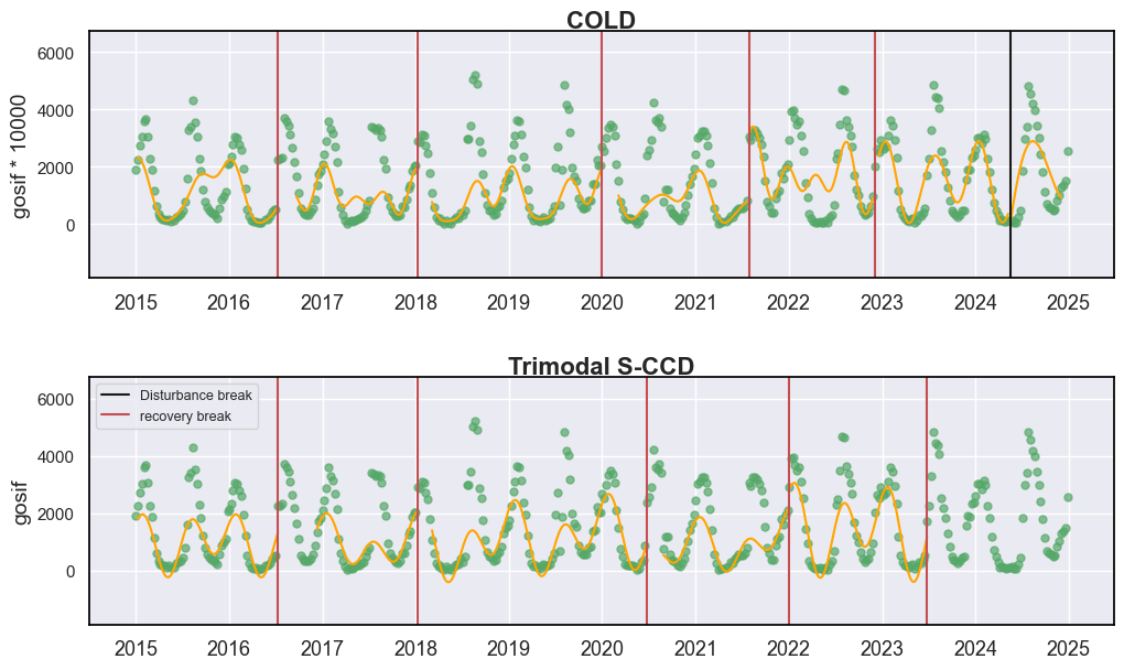
从图中可以观察到,COLD 和 S-CCD 算法得出的结果有些不同。然而,两种方法都未能捕捉到先前研究报告的 2020 年和 2022 年与干旱相关的断点。这种遗漏可能是因为数据集的空间分辨率较粗,倾向于平滑时间信号,从而减弱了短期波动的幅度,并降低了干旱引起变化的统计显著性。
提高检测断点的灵敏度
让我们尝试使用激进的参数设置(p_cg=0.9; conse=3)进行断点检测:
# we applied an aggressive parameter set
sccd_result = sccd_detect_flex(dates, sif, qas, p_cg=0.9, conse=3, trimodal=True, lam=20, fitting_coefs=True)
cold_result = cold_detect_flex(dates, sif, qas,  p_cg=0.9, conse=3, lam=20)

# Set up plotting style
sns.set_theme(style="darkgrid")
sns.set_context("notebook")

# plot time series and detection results
fig, axes = plt.subplots(2, 1, figsize=(12, 7))
plt.subplots_adjust(hspace=0.4)

display_cold_result_sif(data=data[(data['GOSIF'] >= 0)].to_numpy(), band_names=['gosif'], band_index=0, cold_result=cold_result, axe=axes[0], title="COLD (0.9, 3)")

display_sccd_result_single(data=data[(data['GOSIF'] >= 0)].to_numpy(), band_names=['gosif'], band_index=0, sccd_result=sccd_result, axe=axes[1], trimodal=True, title="Trimodal S-CCD (0.9, 3)")
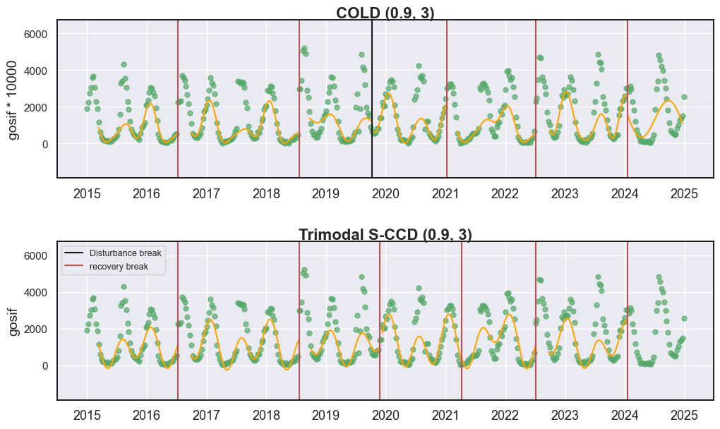
现在,我们可以看到两种算法都检测到了更多的断点。然而,其中大部分归因于恢复(即 GOSIF 增加)。
尽管频繁的“断点”检测对于捕捉快速变化可能看起来是可取的,但这 对于类似 CCDC 的算法来说并不一定有利。过多的断点检测会频繁触发模型重新初始化,这会引入至少一年的监测间隙,从而限制检测连续干扰的能力。此外,每个时间段观察期的缩短降低了模型拟合的稳健性和准确性。频繁的重新初始化也使得近实时(NRT)监测复杂化,因为在新时间段内缺乏稳定的模型会破坏时间连续性。然而,在实践中,重新初始化仍然是必要的,因为与大量土地覆盖转换相关的结构变化会在模型系数中引入较大的不确定性,从而需要进行模型重新校准。
解决方案:“异常-断点”二级检测
为了解决这个问题,S-CCD 允许采用一个**双层层级框架**来区分异常和断点。异常是指在相对较短的时间窗口内,以较小的幅度阈值偏离模型预测的观测值。相比之下,断点代表具有较大偏差和延长时间的特征的异常集群,表明时间序列中发生了结构变化。当检测到异常时,S-CCD 会记录关键参数(例如 t_break、谐波系数、变化幅度),但它不会重新初始化模型。只有在确认发生断点时,S-CCD 才会执行模型重新初始化。
Name |
Definition |
Default parameters |
Re-initialization |
Usage |
|---|---|---|---|---|
Anomalies |
Observations that deviate from the predicted |
|
No |
|
Breaks |
Observations that cause structural changes |
|
Yes |
|
sccd_result1 = sccd_detect_flex(dates, sif, qas,  p_cg=0.9, conse=3, trimodal=True, lam=20)

# we turned on the anomaly output
sccd_result2, anomaly = sccd_detect_flex(dates, sif, qas, p_cg = 0.9999, conse=8, output_anomaly=True, trimodal=True, lam=20, fitting_coefs=True)


# Set up plotting style
sns.set_theme(style="darkgrid")
sns.set_context("notebook")

# plot time series and detection results
fig, axes = plt.subplots(2, 1, figsize=(12, 7))
plt.subplots_adjust(hspace=0.4)

display_sccd_result_single(data=data[(data['GOSIF'] >= 0)].to_numpy(), band_names=['gosif'], band_index=0, sccd_result=sccd_result1, axe=axes[0], trimodal=True, title="Trimodal S-CCD (0.9, 3)")

display_sccd_result_single(data=data[(data['GOSIF'] >= 0)].to_numpy(), band_names=['gosif'], band_index=0, sccd_result=sccd_result2, axe=axes[1], trimodal=True, anomaly=anomaly, title="Trimodal S-CCD with anomalies (0.9, 3)")
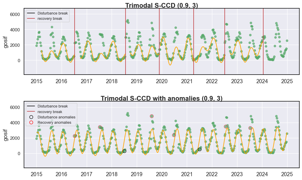
检测到的异常在上图中以圆圈高亮显示。我们发现,它与使用相同参数设置(conse=3,p_cg=0.9)检测到的断点存在中等程度的差异,这证明了**频繁的初始化确实会影响断点检测**。异常提供了更准确的检测,例如,2021 年的显著下降已被 Trimodal S-CCD with anomalies (0.9, 3) 捕捉到,但在仅依赖断点检测而非“异常-断点”二级检测的 Trimodal S-CCD (0.9, 3) 中却被遗漏了。
输出 anomaly 存储了每个被检测异常的大量信息,这些信息可用于机器学习,并可进一步用于近实时干扰监测 [3]。
[3] Ye, S., Zhu, Z., & Suh, J. W. (2024). Leveraging past information and machine learning to accelerate land disturbance monitoring. Remote Sensing of Environment, 305, 114071.
print(anomaly)
SccdReccganomaly(position=1, rec_cg_anomaly=array([(736156, [[ 5.1858328e+04, -6.9177362e+02,  3.3654770e+02, -1.7499992e+01,  9.5840057e+02,  8.6213184e+02,  5.0908569e+02, -8.8351173e+01]], [[2246, 2269, 2317, 3703, 3604, 3441, 3108, 2656]], [12414, 12422, 12430, 12438, 12446, 12454, 12462, 12470], [2045, 1376,  866,  866,  866,  866,  866,  619], [    0,     0,     0,     0,     0,     0,     0,     0]),
       (736522, [[-9.6152391e+04,  1.3227594e+03,  2.4489276e+02, -2.7984451e+02,  9.8913678e+02,  9.1183948e+02,  4.3716653e+02, -1.6476933e+02]], [[3405, 3365, 3288, 3343, 3275, 3053, 2240, 1924]], [12780, 12788, 12796, 12804, 12812, 12820, 12828, 12836], [2350, 1521,  834,  529,  261,   69,   69,   69], [    0,     0,     0,     0,     0,     0,  3000,  2571]),
       (736879, [[-6.8156734e+04,  9.4231702e+02,  2.4477156e+02, -3.1494083e+02,  1.0485380e+03,  8.3385455e+02,  3.3004968e+02, -2.2306662e+02]], [[ 308,  483, 2969, 2970, 3449, 5039, 5201, 4901]], [13137, 13145, 13153, 13161, 13169, 13177, 13185, 13193], [ 366,  366,  366,  272,  272,  272,  272,  272], [    0,     0,  9000,  6000,  4500,  3600,  3000,  2571]),
       (737276, [[-9.1336836e+04,  1.2574849e+03,  2.4061501e+02, -3.2586148e+02,  1.0368047e+03,  8.8601984e+02,  3.2224103e+02, -1.7332237e+02]], [[4836, 4175, 4022, 3194, 1973, 1644, 1507,  874]], [13534, 13542, 13550, 13558, 13566, 13574, 13582, 13590], [2228,  886,  644,   93,   93,   93,   38,   38], [    0,     0,     0,     0,  4500,  3600,  3000,  2571]),
       (737601, [[-1.1669240e+05,  1.6021804e+03,  2.4623053e+02, -3.6994354e+02,  1.0732014e+03,  8.6004553e+02,  2.9123221e+02, -1.9354453e+02]], [[2387, 2577, 2918, 4221, 3616, 3538, 3716, 3410]], [13859, 13867, 13875, 13883, 13891, 13899, 13907, 13915], [ 783,  601,  564,  564,  557,  273,  273,   92], [    0,     0,     0,     0,     0,     0,     0,     0]),
       (737975, [[-1.0452194e+05,  1.4368601e+03,  1.7325824e+02, -3.4035739e+02,  1.1939840e+03,  8.3038953e+02,  2.1778127e+02, -2.0333830e+02]], [[ 531,  608,  801, 3064, 2935, 3238, 3260, 3161]], [14233, 14241, 14249, 14257, 14265, 14273, 14281, 14289], [ 514,  514,  514,   32,    0,    0,    0,    0], [    0,     0,     0,  6000,  9000, 10800,  9000,  7714]),
       (738356, [[-1.0974823e+05,  1.5078867e+03,  2.3844513e+02, -4.0255188e+02,  1.1809484e+03,  8.5556641e+02,  2.7895740e+02, -1.9610316e+02]], [[3481, 4695, 4649, 3642, 3377, 3081, 2682, 1695]], [14614, 14622, 14630, 14638, 14646, 14654, 14662, 14670], [ 429,  429,  429,  108,   27,    4,    0,    0], [    0,     0,     0,     0,     0,     0,  3000,  2571]),
       (738713, [[-1.1450325e+05,  1.5725342e+03,  1.9035295e+02, -4.3067133e+02,  1.2565746e+03,  8.3714301e+02,  2.3216125e+02, -2.4270714e+02]], [[3278, 4839, 4437, 4380, 4058, 2532, 2176, 1816]], [14971, 14979, 14987, 14995, 15003, 15011, 15019, 15027], [ 384,  384,  384,  384,  198,  197,  197,  197], [    0,     0,     0,     0,     0,  3600,  3000,  2571])],
      dtype={'names': ['t_break', 'coefs', 'obs', 'obs_date_since1982', 'norm_cm', 'cm_angle'], 'formats': ['<i4', ('<f4', (1, 8)), ('<i2', (1, 8)), ('<i2', (8,)), ('<i2', (8,)), ('<i2', (8,))], 'offsets': [0, 4, 36, 52, 68, 84], 'itemsize': 100, 'aligned': True}))
S-CCD 还允许用户通过调整 anomaly_conse 和 anomaly_pcg 来定义异常:
sccd_result1 = sccd_detect_flex(dates, sif, qas,  p_cg=0.95, conse=4, lam=20)
sccd_result2, anomaly = sccd_detect_flex(dates, sif, qas, anomaly_conse=4, anomaly_pcg=0.95, p_cg = 0.9999, output_anomaly=True, trimodal=True, lam=20, fitting_coefs=True)


# Set up plotting style
sns.set_theme(style="darkgrid")
sns.set_context("notebook")

# plot time series and detection results
fig, axes = plt.subplots(2, 1, figsize=(12, 7))
plt.subplots_adjust(hspace=0.4)

display_sccd_result_single(data=data[(data['GOSIF'] >= 0)].to_numpy(), band_names=['gosif'], band_index=0, sccd_result=sccd_result1, axe=axes[0], trimodal=True, title="Trimodal S-CCD (0.95, 4)")

display_sccd_result_single(data=data[(data['GOSIF'] >= 0)].to_numpy(), band_names=['gosif'], band_index=0, sccd_result=sccd_result2, axe=axes[1], anomaly=anomaly, trimodal=True, title="Trimodal S-CCD with anomalies (0.95, 4)")
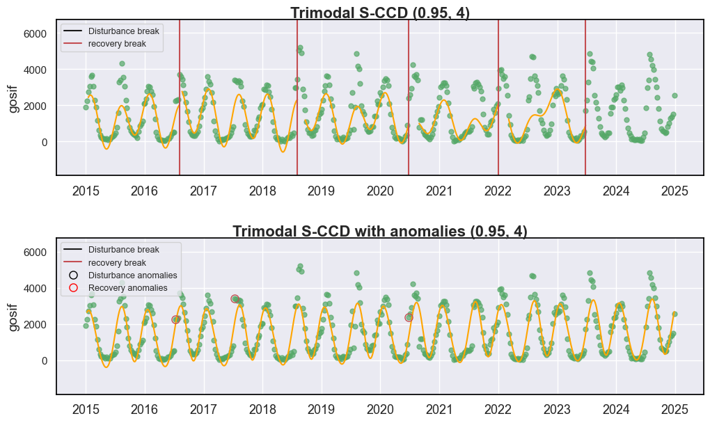
现在你可以看到,在“Trimodal S-CCD with anomalies (0.95, 4)”中,“Trimodal S-CCD with anomalies (0.90, 3)”检测到的所有干旱信号都消失了。
值得注意的是,S-CCD 主要是为了检测植被时间序列中的绿化或褐化异常而设计的,而不是将这些异常归因于特定的成因因素。识别出的异常代表了与预测时间轨迹的显著偏离,但它们不一定表明是由干旱胁迫引起的。这种植被变化也可能源于其他驱动因素,包括土地用途转换、病虫害爆发或与水分可用性无关的气候波动。因此,为了确认检测到的异常是否确实是干旱驱动的,建议**将分析与独立的标准化降水蒸散指数(SPEI)时间序列相结合**。这种补充评估有助于在植被异常与气象干旱条件之间建立更直接的联系,从而提高干旱归因和解释的可靠性。