第2课：参数设置

作者: 叶粟 (remotesensingsuy@gmail.com)

时间序列数据集: Landsat 5,7,8 数据集

应用: 美国科罗拉多州和马萨诸塞州的昆虫干扰

虽然类似 CCDC 的算法的默认参数已经过严格验证，但对于某些特定干扰类型，其性能可能并非最佳。本课程将展示不同参数设置对检测干扰的影响，从而为 COLD/S-CCD 的参数设置提供指导。

---

变化概率

类似 CCDC 的方法中一个重要的参数是变化概率（p_cg）。COLD/S-CCD 通过将所有涉及光谱波段的变化幅度组合成一个范数来确定断点。从统计学上讲，变化幅度向量的范数服从卡方（chi-square）分布。参数 p_cg 指定了用于定义该分布临界值的概率水平，从而决定了观测值必须偏离预测的 COLD/S-CCD 曲线多少才能被标记为断点的阈值。

山松甲虫（Mountain Pine Beetle, MPB）的爆发在科罗拉多州的落基山脉造成了广泛的树木死亡，大约始于 2003 年，并在 2007 年达到顶峰。侵染后，受攻击的树木通常保持绿色约一年（”绿色阶段”），然后在接下来的一年内随着针叶失去叶绿素而变为红色，并最终随着落叶的发生进入灰色阶段。基于遥感的 MPB 监测面临的一个主要挑战是，初始侵染阶段的光谱变化幅度通常很细微，因为针叶大部分保持完整且仍为绿色。因此，S-CCD/COLD 中默认的干扰检测阈值（例如，p_cg = 0.99，这是为捕捉一般性干扰事件而校准的）可能不足以灵敏地识别与甲虫活动相关的早期光谱信号。

我们将使用美国科罗拉多州一个受 MPB 影响的地点的基于 Landsat 的时间序列来演示使用 S-CCD 进行干扰监测。

默认参数

import numpy as np
import pathlib
import pandas as pd

# Imports from this package
from pyxccd import sccd_detect


TUTORIAL_DATASET = (pathlib.Path.cwd() / 'datasets').resolve() # modify it as you need
assert TUTORIAL_DATASET.exists()
in_path = TUTORIAL_DATASET/ '2_mpb_co_landsat.csv' # read the MPB-affected plot in CO

# read example csv for HLS time series
data = pd.read_csv(in_path)

# split the array by the column
dates, blues, greens, reds, nirs, swir1s, swir2s, thermals, qas, sensor = data.to_numpy().copy().T
sccd_result = sccd_detect(dates, blues, greens, reds, nirs, swir1s, swir2s, qas, p_cg=0.999)

sccd_result.rec_cg

array([], dtype=float64)

变化记录 rec_cg 为空，这意味着 S-CCD 使用默认参数没有检测到任何断点。让我们深入分析使用短波红外2（SWIR2）的时间序列，这是对水分胁迫最敏感的波段：

from datetime import date
from typing import List, Tuple, Dict, Union, Optional
import seaborn as sns
import matplotlib.pyplot as plt
from matplotlib.axes import Axes
from pyxccd.common import SccdOutput
from pyxccd.utils import getcategory_sccd, defaults

def display_sccd_result(
    data: np.ndarray,
    band_names: List[str],
    band_index: int,
    sccd_result: SccdOutput,
    axe: Axes,
    title: str = 'S-CCD',
    plot_kwargs: Optional[Dict] = None
) -> Tuple[plt.Figure, List[plt.Axes]]:
    """
    Compare COLD and SCCD change detection algorithms by plotting their results side by side.

    This function takes time series remote sensing data, applies both COLD and SCCD algorithms,
    and visualizes the curve fitting and break detection results for comparison.

    Parameters:
    -----------
    data : np.ndarray
        Input data array with shape (n_observations, n_bands + 2) where:
        - First column: ordinal dates (days since January 1, AD 1)
        - Next n_bands columns: spectral band values
        - Last column: QA flags (0-clear, 1-water, 2-shadow, 3-snow, 4-cloud)

    band_names : List[str]
        List of band names corresponding to the spectral bands in the data (e.g., ['red', 'nir'])

    band_index : int
        1-based index of the band to plot (e.g., 0 for first band, 1 for second band)

    sccd_result: SccdOutput
        Output of sccd_detect

    axe: Axes
        An Axes object represents a single plot within that Figure

    title: Str
        The figure title. The default is "S-CCD"

    plot_kwargs : Dict, optional
        Additional keyword arguments to pass to the display function. Possible keys:
        - 'marker_size': size of observation markers (default: 5)
        - 'marker_alpha': transparency of markers (default: 0.7)
        - 'line_color': color of model fit lines (default: 'orange')
        - 'font_size': base font size (default: 14)

    Returns:
    --------
    Tuple[plt.Figure, List[plt.Axes]]
        A tuple containing the matplotlib Figure object and a list of Axes objects
        (top axis is COLD results, bottom axis is SCCD results)

    """
    w = np.pi * 2 / 365.25

    # Set default plot parameters
    default_plot_kwargs: Dict[str, Union[int, float, str]] = {
        'marker_size': 5,
        'marker_alpha': 0.7,
        'line_color': 'orange',
        'font_size': 14
    }
    if plot_kwargs is not None:
        default_plot_kwargs.update(plot_kwargs)

    # Extract values with proper type casting
    font_size = default_plot_kwargs.get('font_size', 14)
    try:
        title_font_size = int(font_size) + 2
    except (TypeError, ValueError):
        title_font_size = 16


    # Clean and prepare data
    data = data[np.all(np.isfinite(data), axis=1)]
    data_df = pd.DataFrame(data, columns=['dates'] + band_names + ['qa'])


    # Plot COLD results
    w = np.pi * 2 / 365.25
    slope_scale = 10000

    # Prepare clean data for COLD plot
    data_clean = data_df[(data_df['qa'] == 0) | (data_df['qa'] == 1)].copy()
    data_clean =  data_clean[(data_clean >= 0).all(axis=1) & (data_clean.drop(columns="dates") <= 10000).all(axis=1)]
    calendar_dates = [pd.Timestamp.fromordinal(int(row)) for row in data_clean["dates"]]
    data_clean.loc[:, 'dates_formal'] = calendar_dates

    # Calculate y-axis limits
    band_name = band_names[band_index]
    band_values = data_clean[data_clean['qa'] == 0 | (data_clean['qa'] == 1)][band_name]
    # band_values  = band_values[band_values <10000]
    q01, q99 = np.quantile(band_values, [0.01, 0.99])
    extra = (q99 - q01) * 0.4
    ylim_low = q01 - extra
    ylim_high = q99 + extra

    # Plot SCCD observations
    axe.plot(
        'dates_formal', band_name, 'go',
        markersize=default_plot_kwargs['marker_size'],
        alpha=default_plot_kwargs['marker_alpha'],
        data=data_clean
    )

    # Plot SCCD segments
    for segment in sccd_result.rec_cg:
        j = np.arange(segment['t_start'], segment['t_break'] + 1, 1)
        if len(segment['coefs'][band_index]) == 8:
            plot_df = pd.DataFrame(
                {
                'dates': j,
                'trend': j * segment['coefs'][band_index][1] / slope_scale + segment['coefs'][band_index][0],
                'annual': np.cos(w * j) * segment['coefs'][band_index][2] + np.sin(w * j) * segment['coefs'][band_index][3],
                'semiannual': np.cos(2 * w * j) * segment['coefs'][band_index][4] + np.sin(2 * w * j) * segment['coefs'][band_index][5],
                'trimodal': np.cos(3 * w * j) * segment['coefs'][band_index][6] + np.sin(3 * w * j) * segment['coefs'][band_index][7]
            })
        else:
            plot_df = pd.DataFrame(
                {
                'dates': j,
                'trend': j * segment['coefs'][band_index][1] / slope_scale + segment['coefs'][band_index][0],
                'annual': np.cos(w * j) * segment['coefs'][band_index][2] + np.sin(w * j) * segment['coefs'][band_index][3],
                'semiannual': np.cos(2 * w * j) * segment['coefs'][band_index][4] + np.sin(2 * w * j) * segment['coefs'][band_index][5],
                'trimodal': j * 0
            })
        plot_df['predicted'] = (
            plot_df['trend'] +
            plot_df['annual'] +
            plot_df['semiannual']+
            plot_df['trimodal']
        )

        # Convert dates and plot model fit
        calendar_dates = [pd.Timestamp.fromordinal(int(row)) for row in plot_df["dates"]]
        plot_df.loc[:, 'dates_formal'] = calendar_dates
        g = sns.lineplot(
            x="dates_formal", y="predicted",
            data=plot_df,
            label="Model fit",
            ax=axe,
            color=default_plot_kwargs['line_color']
        )
        if g.legend_ is not None:
            g.legend_.remove()

    # Plot near-real-time projection for SCCD if available
    if hasattr(sccd_result, 'nrt_mode') and (sccd_result.nrt_mode %10 == 1 or sccd_result.nrt_mode == 3 or sccd_result.nrt_mode %10 == 5):
        recent_obs = sccd_result.nrt_model['obs_date_since1982'][sccd_result.nrt_model['obs_date_since1982']>0]
        j = np.arange(
            sccd_result.nrt_model['t_start_since1982'].item() + defaults['COMMON']['JULIAN_LANDSAT4_LAUNCH'],
            recent_obs[-1].item()+ defaults['COMMON']['JULIAN_LANDSAT4_LAUNCH']+1,
            1
        )

        if len(sccd_result.nrt_model['nrt_coefs'][band_index]) == 8:
            plot_df = pd.DataFrame(
                {
                'dates': j,
                'trend': j * sccd_result.nrt_model['nrt_coefs'][band_index][1] / slope_scale + sccd_result.nrt_model['nrt_coefs'][band_index][0],
                'annual': np.cos(w * j) * sccd_result.nrt_model['nrt_coefs'][band_index][2] + np.sin(w * j) * sccd_result.nrt_model['nrt_coefs'][band_index][3],
                'semiannual': np.cos(2 * w * j) * sccd_result.nrt_model['nrt_coefs'][band_index][4] + np.sin(2 * w * j) * sccd_result.nrt_model['nrt_coefs'][band_index][5],
                'trimodal': np.cos(3 * w * j) * sccd_result.nrt_model['nrt_coefs'][band_index][6] + np.sin(3 * w * j) * sccd_result.nrt_model['nrt_coefs'][band_index][7]
            })
        else:
            plot_df = pd.DataFrame(
                {
                'dates': j,
                'trend': j * sccd_result.nrt_model['nrt_coefs'][band_index][1] / slope_scale + sccd_result.nrt_model['nrt_coefs'][band_index][0],
                'annual': np.cos(w * j) * sccd_result.nrt_model['nrt_coefs'][band_index][2] + np.sin(w * j) * sccd_result.nrt_model['nrt_coefs'][band_index][3],
                'semiannual': np.cos(2 * w * j) * sccd_result.nrt_model['nrt_coefs'][band_index][4] + np.sin(2 * w * j) * sccd_result.nrt_model['nrt_coefs'][band_index][5],
                'trimodal': j * 0
            })

        plot_df['predicted'] = plot_df['trend'] + plot_df['annual'] + plot_df['semiannual']+ plot_df['trimodal']
        calendar_dates = [pd.Timestamp.fromordinal(int(row)) for row in plot_df["dates"]]
        plot_df.loc[:, 'dates_formal'] = calendar_dates
        g = sns.lineplot(
            x="dates_formal", y="predicted",
            data=plot_df,
            label="Model fit",
            ax=axe,
            color=default_plot_kwargs['line_color']
        )
        if g.legend_ is not None:
            g.legend_.remove()

    # Plot breaks
    for i in range(len(sccd_result.rec_cg)):
        if getcategory_sccd(sccd_result.rec_cg, i) == 1:
            axe.axvline(pd.Timestamp.fromordinal(sccd_result.rec_cg[i]['t_break']), color='k')
        else:
            axe.axvline(pd.Timestamp.fromordinal(sccd_result.rec_cg[i]['t_break']), color='r')

    axe.set_ylabel(f"{band_name} * 10000", fontsize=default_plot_kwargs['font_size'])

    # Handle tick params with type safety
    tick_font_size = default_plot_kwargs['font_size']
    if isinstance(tick_font_size, (int, float)):
        axe.tick_params(axis='x', labelsize=int(tick_font_size)-1)
    else:
        axe.tick_params(axis='x', labelsize=13)  # fallback

    axe.set(ylim=(ylim_low, ylim_high))
    axe.set_xlabel("", fontsize=6)

    # Format spines
    for spine in axe.spines.values():
        spine.set_edgecolor('black')
    axe.set_title(title, fontweight="bold", size=title_font_size, pad=2)

sns.set_theme(style="darkgrid")
sns.set_context("notebook")

# Create figure and axes
fig, ax = plt.subplots(figsize=(12, 5))

display_sccd_result(data=np.stack((dates, blues, greens, reds, nirs, swir1s, swir2s, thermals, qas), axis=1), band_names=['blues', 'green', 'red', 'nir', 'swir1', 'swir2', 'thermals'], band_index=5, sccd_result=sccd_result, axe=ax, title="Standard S-CCD")

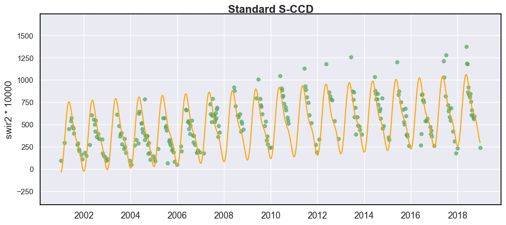
从图中可以观察到短波红外波段存在上升趋势，表明水分胁迫加剧，尽管 S-CCD 没有检测到任何断点。这种上升趋势是该像元受甲虫攻击的信号。

信号分解

为了验证这个视觉上识别的趋势，我们将检查 S-CCD 提供的 states 工具。在状态空间模型的上下文中，状态表示时间 \(t+1\) 时波段 \(i\) 的地表信号状况，可以递归地更新时间 \(t\) 的滤波状态 \(a_{t|t,i}\)：

\[a_{t+1,i}=Ta_{t|t,i}\]

其中 \(T\) 是一个转换矩阵。对于每个波段，states \(a\) 包含三个随时间变化的元素：趋势、年际、半年际和三级谐波（如果可用）。这些 states 支持对季节性、长期趋势和其他动态进行时间段内分析，从而补充了 S-CCD 检测到的光谱断点。我们将在第 5 课中详细介绍 state analysis。

为了输出状态，用户只需在 sccd_detect 函数中将参数 state_intervaldays 设置为非零整数（通常设为 1，表示状态按日输出），sccd_detect 将生成 S-CCD 常规输出的结构化对象以及额外的状态记录：

def display_sccd_states_flex(
    data_df: pd.DataFrame,
    states:pd.DataFrame,
    axes: Axes,
    variable_name: str,
    title:str,
    band_name:str = "b0",
    plot_kwargs: Optional[Dict] = None
):
    default_plot_kwargs: Dict[str, Union[int, float, str]] = {
        'marker_size': 5,
        'marker_alpha': 0.7,
        'line_color': 'orange',
        'font_size': 14
    }
    if plot_kwargs is not None:
        default_plot_kwargs.update(plot_kwargs)

    # convert ordinal dates to calendar
    formal_dates = [pd.Timestamp.fromordinal(int(row)) for row in states["dates"]]
    states.loc[:, "dates_formal"] = formal_dates

    extra = (np.max(states[f"{band_name}_trend"]) - np.min(states[f"{band_name}_trend"])) / 4
    axes[0].set(ylim=(np.min(states[f"{band_name}_trend"]) - extra, np.max(states[f"{band_name}_trend"]) + extra))
    sns.lineplot(x="dates_formal", y=f"{band_name}_trend", data=states, ax=axes[0], color="orange")
    axes[0].set(ylabel=f"Trend")

    extra = (np.max(states[f"{band_name}_annual"]) - np.min(states[f"{band_name}_annual"])) / 4
    axes[1].set(ylim=(np.min(states[f"{band_name}_annual"]) - extra, np.max(states[f"{band_name}_annual"]) + extra))
    sns.lineplot(x="dates_formal", y=f"{band_name}_annual", data=states, ax=axes[1], color="orange")
    axes[1].set(ylabel=f"Annual cycle")

    extra = (np.max(states[f"{band_name}_semiannual"]) - np.min(states[f"{band_name}_semiannual"])) / 4
    axes[2].set(ylim=(np.min(states[f"{band_name}_semiannual"]) - extra, np.max(states[f"{band_name}_semiannual"]) + extra))
    sns.lineplot(x="dates_formal", y=f"{band_name}_semiannual", data=states, ax=axes[2], color="orange")
    axes[2].set(ylabel=f"Semi-annual cycle")


    data_clean = data_df[(data_df["qa"] == 0) | (data_df['qa'] == 1)].copy() # CCDC also processes water pixels
    formal_dates = [pd.Timestamp.fromordinal(int(row)) for row in data_clean["dates"]]
    data_clean.loc[:, "dates_formal"] = formal_dates  # convert ordinal dates to calendar
    axes[3].plot(
        'dates_formal', variable_name, 'go',
        markersize=default_plot_kwargs['marker_size'],
        alpha=default_plot_kwargs['marker_alpha'],
        data=data_clean
    )

    states["General"] = states[f"{band_name}_annual"] + states[f"{band_name}_trend"] + states[f"{band_name}_semiannual"]
    g = sns.lineplot(
        x="dates_formal", y="General", data=states, label="fit", ax=axes[3], color="orange"
    )

    axes[3].set_ylabel(f"{variable_name}", fontsize=default_plot_kwargs['font_size'])
    axes[3].set_title(title, fontweight="bold", size=16 , pad=2)

    band_values = data_df[data_df['qa'] == 0][variable_name]
    q01, q99 = np.quantile(band_values, [0.01, 0.99])
    extra = (q99 - q01) * 0.4
    ylim_low = q01 - extra
    ylim_high = q99 + extra
    axes[3].set(ylim=(ylim_low, ylim_high))



# Set up plotting style
sns.set_theme(style="darkgrid")
sns.set_context("notebook")

# Create figure and axes
fig, axes = plt.subplots(4, 1, figsize=[12, 10], sharex=True)
plt.subplots_adjust(left=0.08, right=0.98, top=0.92, bottom=0.1)

# specify state_intervaldays as a non-zero value to output states
sccd_result, states = sccd_detect(dates, blues, greens, reds, nirs, swir1s, swir2s, qas, state_intervaldays=1)
display_sccd_states_flex(data_df=data, axes=axes,states=states, band_name="swir2", variable_name="swir2", title="S-CCD")

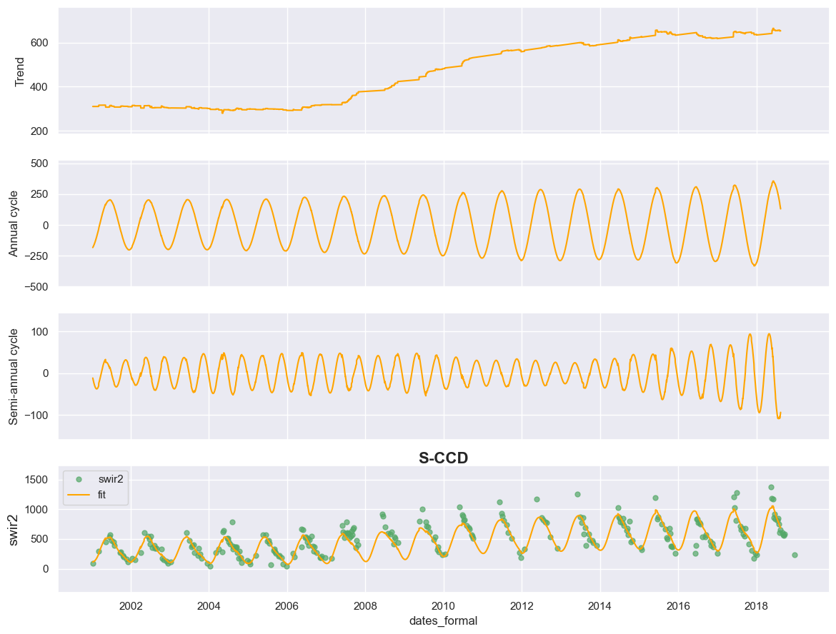
从 Trend 分量（第一个子图）中，我们识别出短波红外2（SWIR2）的一个显著上升趋势，这证实了该森林像元受到了甲虫攻击。初始的抬升信号大约出现在 2007 年左右。

调整 p_cg

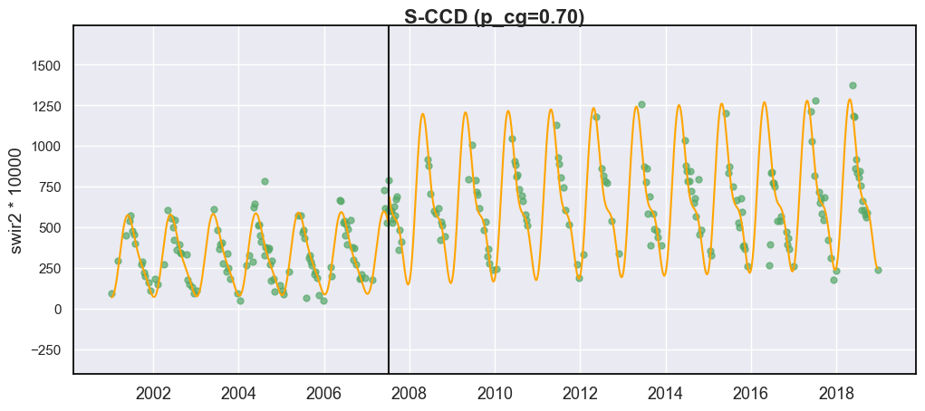
现在我们尝试通过将 p_cg 调整为一个更低的值来检测断点。参数 p_cg，代表变化的卡方概率，定义了检测断点的光谱阈值。默认情况下，p_cg 设置为 0.99。在本例中，当我们将 p_cg 降低到 0.7 时，S-CCD 能够更准确地检测到断点。

值得注意的是，检测到了两个断点：第一个被 ``getcategory_sccd``（基于规则集）自动标记为”恢复”，因此用红线标记。

fig, ax = plt.subplots(figsize=(12, 5))


sccd_result = sccd_detect(dates, blues, greens, reds, nirs, swir1s, swir2s, qas, p_cg=0.70)
display_sccd_result(data=np.stack((dates, blues, greens, reds, nirs, swir1s, swir2s, thermals, qas), axis=1), band_names=['blues', 'green', 'red', 'nir', 'swir1', 'swir2', 'thermals'], band_index=5, sccd_result=sccd_result, axe=ax, title="S-CCD (p_cg=0.70)")

连续观测数

S-CCD/COLD 的另一个重要参数是连续偏离预测值且变化幅度超过阈值的观测数量，即 conse。Conse 有时也称为 峰值窗口宽度。conse 的默认值为 6，意味着只有当至少连续六个观测值（一个峰值窗口）被识别为断点观测，且每个观测值引起的光谱变化幅度都大于卡方分布在概率 p_cg 下的临界值时，才会识别一个断点。如果干扰持续时间短且很快恢复（例如干旱、洪水），那么 S-CCD 可能会因为不满足 conse=6 而错过断点。

舞毒蛾（Spongy Moth, SM）就是这样一种短暂的食叶昆虫，原产于欧洲和亚洲，于 1869 年意外引入马萨诸塞州。在新英格兰地区，舞毒蛾的爆发是间歇性的但很严重，由气候、寄主（橡树优势度）和天敌之间的相互作用驱动。2015-2018 年的爆发突显了干旱如何使天平向昆虫种群爆发倾斜，导致大规模的森林落叶和树木死亡率升高。舞毒蛾通常在 4 月下旬孵化，6 月下旬化蛹导致落叶，这引起近红外（NIR）显著下降，但许多硬木（橡树、枫树、桦树）会在 7 月下旬或 8 月重新长叶，使其成为一种典型的短暂干扰。

NIR 与 SWIR2 对比

让我们使用 S-CCD 的默认参数来检测美国马萨诸塞州的一个舞毒蛾点，并用 NIR 和 SWIR2 波段绘制结果：

in_path = TUTORIAL_DATASET/ '2_sm_ma_landsat.csv' # read the MPB-affected plot in CO

# read example csv for HLS time series
data = pd.read_csv(in_path)

dates, blues, greens, reds, nirs, swir1s, swir2s, thermals, qas, sensor = data.to_numpy().copy().T

# using the default parameters
sccd_result = sccd_detect(dates, blues, greens, reds, nirs, swir1s, swir2s, qas)

# plot time series and detection results
fig, axes = plt.subplots(2, 1, figsize=(12, 7))
plt.subplots_adjust(hspace=0.4)

display_sccd_result(data=np.stack((dates, blues, greens, reds, nirs, swir1s, swir2s, thermals, qas), axis=1), band_names=['blues', 'green', 'red', 'nir', 'swir1', 'swir2', 'thermals'], band_index=5, sccd_result=sccd_result, axe=axes[0], title="Standard S-CCD")

display_sccd_result(data=np.stack((dates, blues, greens, reds, nirs, swir1s, swir2s, thermals, qas), axis=1), band_names=['blues', 'green', 'red', 'nir', 'swir1', 'swir2', 'thermals'], band_index=3, sccd_result=sccd_result, axe=axes[1], title="Standard S-CCD")

这里有两个发现。1）我们可以观察到 2017 年夏季 NIR 的明显下降，而 SWIR2 的变化信号并不像 MPB 那样直接，这反映了树木对食叶害虫和蛀干害虫（蛀干害虫在植物木质部内部钻洞和取食）的不同生理反应。2）从时间序列可以直观地看出 2017 年存在 NIR 下降，但由于干扰持续时间太短，S-CCD 未能检测到它。

调整 conse

让我们调整一下 conse：

# lowering conse to 4
sccd_result = sccd_detect(dates, blues, greens, reds, nirs, swir1s, swir2s, qas, conse=4)

# plot time series and detection results
fig, axes = plt.subplots(2, 1, figsize=(12, 7))
plt.subplots_adjust(hspace=0.4)

display_sccd_result(data=np.stack((dates, blues, greens, reds, nirs, swir1s, swir2s, thermals, qas), axis=1), band_names=['blues', 'green', 'red', 'nir', 'swir1', 'swir2', 'thermals'], band_index=5, sccd_result=sccd_result, axe=axes[0], title="S-CCD (conse=4)")

display_sccd_result(data=np.stack((dates, blues, greens, reds, nirs, swir1s, swir2s, thermals, qas), axis=1), band_names=['blues', 'green', 'red', 'nir', 'swir1', 'swir2', 'thermals'], band_index=3, sccd_result=sccd_result, axe=axes[1], title="S-CCD (conse=4)")

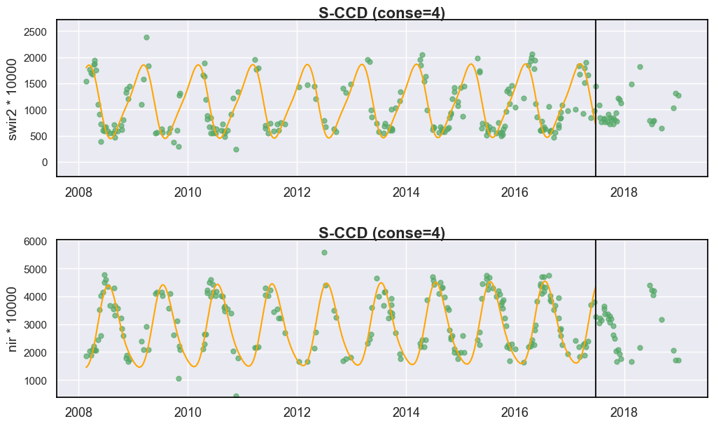
通过将 conse 从 6 降低到 4，我们成功地检测到了由舞毒蛾侵染引起的光谱断点。值得注意的是，标准 S-CCD/COLD 基于五个光谱波段（绿、红、近红外、短波红外1、短波红外2）的组合变化幅度来识别单个断点。因此，所有五个波段共享相同的断点，即使短波红外2 波段没有表现出明显的光谱变化。

在这种情况下，第二个时间段没有可用的曲线拟合，因为没有足够的观测值来初始化近实时（NRT）模型。为了验证这一点，可以检查 nrt_mode 的第二位：值为 2 表示模型尚未初始化，而值为 1 表示有可用的 NRT 模型。

print(f"The second digit of nrt_mode is {sccd_result.nrt_mode % 10}")

The second digit of nrt_mode is 2

总结

降低 conse 和 p_cg 可以提高断点检测的灵敏度，因为需要更少的连续异常观测值或更低的变化幅度阈值来标记变化。然而，这种调整也增加了误报（虚警错误）的可能性，短期噪声或与天气相关的异常可能会被误分类为断点。因此，应仔细调整 conse 和 p_cg。当目标是捕捉细微的地表变化时，建议进行参数敏感性分析。另一个常见策略是应用更激进的参数设置以最大化灵敏度，然后使用机器学习分类器来分离感兴趣的具体变化。