第1课:使用 COLD 和 S-CCD 检测干扰
作者: 叶粟 (remotesensingsuy@gmail.com)
时间序列数据集: Harmonized Landsat-Sentinel (HLS) 数据集
应用: 中国四川的森林火灾
COLD (最新版 CCDC)
连续土地干扰监测(COntinuous monitoring of Land Disturbance, COLD)算法是连续变化检测与分类(Continuous Change Detection and Classification, CCDC)的最新版本,专为使用卫星影像(特别是 Landsat 档案)监测地表动态而开发。COLD 由 Zhe 等人(2020 年)提出,对 Zhe 等人(2014 年)提出的原始 CCDC 进行了一些重要改进。COLD/CCDC 通过用一组捕获季节变化的谐波回归函数(以及表示长期趋势的线性项)拟合所有可用的观测数据,在像元级别模拟地表反射率的时间轨迹。这使得算法能够连续跟踪地表发生的渐近和突变变化。
当新的观测数据到达时,COLD/CCDC 评估它们是否显著偏离建模的轨迹。如果检测到持续偏离超过统计阈值,则会识别出一个断点,表明可能存在干扰或土地覆盖变化事件(检测)。通过记录每个像元的多个断点,COLD/CCDC 支持历史变化的监测,如森林干扰、城市扩张、农业轮作或植被恢复。同时,COLD/CCDC 提取由断点确定的每个时间段(segment)的谐波系数,这些系数将用于基于时间段的土地覆盖分类(分类)。
参考文献:
Zhu, Z., Zhang, J., Yang, Z., Aljaddani, A. H., Cohen, W. B., Qiu, S., & Zhou, C. (2020). Continuous monitoring of land disturbance based on Landsat time series. Remote Sensing of Environment, 238, 111116.
Zhu, Z., & Woodcock, C. E. (2014). Continuous change detection and classification of land cover using all available Landsat data. Remote sensing of Environment, 144, 152-171.
COLD 断点检测
雅安火灾是中国最具破坏性的野火之一,于 3 月 22 日发生在四川省雅安县。下面展示使用 COLD 检测 2024 年雅安火灾下基于像元的 HLS 时间序列:
import numpy as np
import pathlib
import pandas as pd

# Imports from this package
from pyxccd import cold_detect


TUTORIAL_DATASET = (pathlib.Path.cwd() / 'datasets').resolve() # modify it as you need
assert TUTORIAL_DATASET.exists()
in_path = TUTORIAL_DATASET/ '1_hls_sc.csv'

# read example csv for HLS time series
data = pd.read_csv(in_path)

# split the array by the column
dates, blues, greens, reds, nirs, swir1s, swir2s, thermals, qas, sensor = data.to_numpy().copy().T
cold_result = cold_detect(dates, blues, greens, reds, nirs, swir1s, swir2s, thermals, qas)

# convert ordinal date to human readable date
break_date = pd.Timestamp.fromordinal(cold_result[0]["t_break"]).strftime('%Y-%m-%d')
print(f"The break detected is {break_date}")
print("COLD results is: ")
print(cold_result)
The break detected is 2024-03-23
COLD results is:
[(735600, 738960, 738968, 1, 472,  8, 100, [[ 1.6766739e+02,  0.0000000e+00,  0.0000000e+00,  0.0000000e+00,  0.0000000e+00,  0.0000000e+00,  0.0000000e+00,  0.0000000e+00], [ 3.6711215e+02,  0.0000000e+00,  0.0000000e+00,  0.0000000e+00,  0.0000000e+00,  0.0000000e+00,  0.0000000e+00,  0.0000000e+00], [ 3.5981775e+02,  0.0000000e+00,  0.0000000e+00,  0.0000000e+00,  0.0000000e+00,  0.0000000e+00,  0.0000000e+00,  0.0000000e+00], [-1.8439887e+04,  2.7444632e+02,  0.0000000e+00,  0.0000000e+00,  2.4501804e+01, -2.7643259e+01,  6.1835299e+00, -1.1128180e+01], [ 1.2269283e+03,  0.0000000e+00,  0.0000000e+00,  9.2912989e+00,  0.0000000e+00, -1.4118568e+01,  0.0000000e+00, -5.2788010e+00], [ 7.1484528e+02,  0.0000000e+00,  0.0000000e+00,  0.0000000e+00,  0.0000000e+00,  0.0000000e+00,  0.0000000e+00,  0.0000000e+00], [ 0.0000000e+00,  0.0000000e+00,  0.0000000e+00,  0.0000000e+00,  0.0000000e+00,  0.0000000e+00,  0.0000000e+00,  0.0000000e+00]], [ 32.981544,  46.93689 ,  51.279877, 134.50009 , 138.7891  ,  92.00378 ,   0.      ], [ 220.33261,  170.38785,  256.18225, -920.6151 ,  158.78595,  771.6547 ,    0.     ])
 (738968, 739252,      0, 1,  46, 24,   0, [[ 4.3974188e+02,  0.0000000e+00,  7.6601973e+00,  0.0000000e+00,  0.0000000e+00,  0.0000000e+00,  0.0000000e+00,  0.0000000e+00], [-6.6828550e+03,  9.8554466e+01,  3.9433846e+01,  0.0000000e+00,  0.0000000e+00,  0.0000000e+00,  0.0000000e+00,  0.0000000e+00], [ 7.4310809e+02,  0.0000000e+00,  6.7782188e+01,  0.0000000e+00,  0.0000000e+00,  0.0000000e+00,  0.0000000e+00,  0.0000000e+00], [-1.9364056e+05,  2.6346836e+03,  5.6232704e+01,  0.0000000e+00,  0.0000000e+00,  0.0000000e+00,  0.0000000e+00,  0.0000000e+00], [ 1.6937788e+03,  0.0000000e+00,  1.1827483e+02,  5.3090653e+00,  0.0000000e+00,  0.0000000e+00,  0.0000000e+00,  0.0000000e+00], [ 1.6231411e+03,  0.0000000e+00,  1.3118753e+02,  7.0458405e+01,  0.0000000e+00,  0.0000000e+00,  0.0000000e+00,  0.0000000e+00], [ 0.0000000e+00,  0.0000000e+00,  0.0000000e+00,  0.0000000e+00,  0.0000000e+00,  0.0000000e+00,  0.0000000e+00,  0.0000000e+00]], [ 70.27479 ,  64.3015  ,  71.30929 ,  87.261406, 123.548836, 113.304276,   0.      ], [   0.     ,    0.     ,    0.     ,    0.     ,    0.     ,    0.     ,    0.     ])]
COLD 是一种基于像元的算法,其基本输出是由断点定义的输入数据的时间段(segment)。运行 cold_detect 后,输出是一个一维结构数组。数组的长度表示该像元的时间段数量(对于本例,我们得到两个时间段和一个断点)。每个元素包含以下 10 个属性:
t_start: 序列模型开始的序数日期
t_end: 序列模型结束的序数日期
t_break: 检测到断点的序数日期(紧邻 t_end 后的观测)
pos: 使用用户定义的日期代码表示的每个时间序列模型的位置。例如,在第 4 课中,pos = i * n_cols + j,其中 i 是基于 0 的行号,j 是基于 1 的列号,以确保 pos 从 1 开始。对于第 1000 行、第 1 列的 HLS 像元,pos 是 3660 * 1000 + 1。
num_obs: 用于模型估计的清晰观测数
category: 模型估计的质量(使用的模型类型及处理流程)
(first digit)
0 - 正常模型(无变化);
1 - 时间序列模型开始处的变化;
2 - 时间序列模型结束处的变化;
3 - 中间干扰变化;
4 - fmask 失败场景;
5 - 永久性雪场景;
6 - 在用户掩膜外

(second digit)
1 - 模型只有常数项;
4 - 模型有 3 个系数 + 1 个常数项;
6 - 模型有 5 个系数 + 1 个常数项;
8 - 模型有 7 个系数 + 1 个常数项;
change_prob: 像元发生变化的概率(0 到 100 之间)
coefs: 形状为 (7, 8) 的二维数组,包含通过 Lasso 回归获得的多光谱谐波系数。每行对应一个特定的光谱波段,固定顺序如下:蓝、绿、红、近红外、短波红外1、短波红外2 和热红外(分别为行 0 到 6)。
注意:pyxccd 中的斜率系数(位于数组的第二列)已被缩放 10,000 倍,以便在使用 float32 精度时优化存储效率。在使用这些系数进行谐波曲线预测之前,必须通过除以 10,000 将斜率值恢复到原始尺度。
rmse: 形状为 (7,) 的一维数组,预测观测值与实际观测值的多光谱均方根误差
magnitude: 形状为 (7,) 的一维数组,检测到断点后连续观测窗口内模型预测与观测值之间的多光谱中位数差异
COLD 断点分类
顾及到光谱断点不一定与干扰有关,也可能与气候变率、演替甚至数据噪声有关,COLD 算法提供了一个快速的基于规则的解决方案来确定断点的类别(1-干扰,2-再生,3-再造林)。更多细节,请参考 COLD 论文(”Continuous monitoring of land disturbance based on Landsat time series”)中的第 3.3.7 节。
Pyxccd 提供了用于确定断点类别的函数:
from pyxccd.utils import getcategory_cold
print(f"The category for the first break is {getcategory_cold(cold_result, 0)}") # 0 表示第一个断点,1 表示第二个,依此类推
The category for the first break is 1
COLD 可视化
接下来,我们将展示如何绘制近红外(NIR)时间序列和 COLD 断点检测结果(注意 COLD 结合了绿、红、近红外、短波红外1、短波红外2 来确定断点,而我们仅使用近红外波段来示例曲线拟合和断点检测):
from pyxccd.common import cold_rec_cg
from pyxccd.utils import read_data, getcategory_cold

from datetime import date
from typing import List, Tuple, Dict, Union, Optional
import seaborn as sns
import matplotlib.pyplot as plt
from matplotlib.axes import Axes

def display_cold_result(
    data: np.ndarray,
    band_names: List[str],
    band_index: int,
    cold_result: cold_rec_cg,
    axe: Axes,
    title: str = 'COLD',
    plot_kwargs: Optional[Dict] = None
) -> Tuple[plt.Figure, List[plt.Axes]]:
    """
    Compare COLD and SCCD change detection algorithms by plotting their results side by side.

    This function takes time series remote sensing data, applies both COLD algorithms,
    and visualizes the curve fitting and break detection results.

    Parameters:
    -----------
    data : np.ndarray
        Input data array with shape (n_observations, n_bands + 2) where:
        - First column: ordinal dates (days since January 1, AD 1)
        - Next n_bands columns: spectral band values
        - Last column: QA flags (0-clear, 1-water, 2-shadow, 3-snow, 4-cloud)

    band_names : List[str]
        List of band names corresponding to the spectral bands in the data (e.g., ['red', 'nir'])

    band_index : int
        0-based index of the band to plot (e.g., 0 for first band, 1 for second band)

    axe: Axes
        An Axes object represents a single plot within that Figure

    title: Str
        The figure title. The default is "COLD"

    plot_kwargs : Dict, optional
        Additional keyword arguments to pass to the display function. Possible keys:
        - 'marker_size': size of observation markers (default: 5)
        - 'marker_alpha': transparency of markers (default: 0.7)
        - 'line_color': color of model fit lines (default: 'orange')
        - 'font_size': base font size (default: 14)

    Returns:
    --------
    Tuple[plt.Figure, List[plt.Axes]]
        A tuple containing the matplotlib Figure object and a list of Axes objects
        (top axis is COLD results, bottom axis is SCCD results)

    """
    w = np.pi * 2 / 365.25

    # Set default plot parameters
    default_plot_kwargs: Dict[str, Union[int, float, str]] = {
        'marker_size': 5,
        'marker_alpha': 0.7,
        'line_color': 'orange',
        'font_size': 14
    }
    if plot_kwargs is not None:
        default_plot_kwargs.update(plot_kwargs)

    # Extract values with proper type casting
    font_size = default_plot_kwargs.get('font_size', 14)
    try:
        title_font_size = int(font_size) + 2
    except (TypeError, ValueError):
        title_font_size = 16


    # Clean and prepare data
    data = data[np.all(np.isfinite(data), axis=1)]
    data_df = pd.DataFrame(data, columns=['dates'] + band_names + ['qa'])

    # Plot COLD results
    w = np.pi * 2 / 365.25
    slope_scale = 10000

    # Prepare clean data for COLD plot
    data_clean = data_df[(data_df['qa'] == 0) | (data_df['qa'] == 1)].copy()
    data_clean =  data_clean[(data_clean >= 0).all(axis=1) & (data_clean.drop(columns="dates") <= 10000).all(axis=1)]
    calendar_dates = [pd.Timestamp.fromordinal(int(row)) for row in data_clean["dates"]]
    data_clean.loc[:, 'dates_formal'] = calendar_dates

    # Calculate y-axis limits
    band_name = band_names[band_index]
    band_values = data_clean[data_clean['qa'] == 0][band_name]
    q01, q99 = np.quantile(band_values, [0.01, 0.99])
    extra = (q99 - q01) * 0.4
    ylim_low = q01 - extra
    ylim_high = q99 + extra

    # Plot COLD observations
    axe.plot(
        'dates_formal', band_name, 'go',
        markersize=default_plot_kwargs['marker_size'],
        alpha=default_plot_kwargs['marker_alpha'],
        data=data_clean
    )

    # Plot COLD segments
    for segment in cold_result:
        j = np.arange(segment['t_start'], segment['t_end'] + 1, 1)
        plot_df = pd.DataFrame({
            'dates': j,
            'trend': j * segment['coefs'][band_index][1] / slope_scale + segment['coefs'][band_index][0],
            'annual': np.cos(w * j) * segment['coefs'][band_index][2] + np.sin(w * j) * segment['coefs'][band_index][3],
            'semiannual': np.cos(2 * w * j) * segment['coefs'][band_index][4] + np.sin(2 * w * j) * segment['coefs'][band_index][5],
            'trimodel': np.cos(3 * w * j) * segment['coefs'][band_index][6] + np.sin(3 * w * j) * segment['coefs'][band_index ][7]
        })
        plot_df['predicted'] = (
            plot_df['trend'] +
            plot_df['annual'] +
            plot_df['semiannual'] +
            plot_df['trimodel']
        )

        # Convert dates and plot model fit
        calendar_dates = [pd.Timestamp.fromordinal(int(row)) for row in plot_df["dates"]]
        plot_df.loc[:, 'dates_formal'] = calendar_dates
        g = sns.lineplot(
            x="dates_formal", y="predicted",
            data=plot_df,
            label="Model fit",
            ax=axe,
            color=default_plot_kwargs['line_color']
        )
        if g.legend_ is not None:
            g.legend_.remove()

    # plot breaks
    for i in range(len(cold_result)):
        if  cold_result[i]['change_prob'] == 100:
            if getcategory_cold(cold_result, i) == 1:
                axe.axvline(pd.Timestamp.fromordinal(cold_result[i]['t_break']), color='k')
            else:
                axe.axvline(pd.Timestamp.fromordinal(cold_result[i]['t_break']), color='r')

    axe.set_ylabel(f"{band_name} * 10000", fontsize=default_plot_kwargs['font_size'])

    # Handle tick params with type safety
    tick_font_size = default_plot_kwargs['font_size']
    if isinstance(tick_font_size, (int, float)):
        axe.tick_params(axis='x', labelsize=int(tick_font_size)-1)
    else:
        axe.tick_params(axis='x', labelsize=13)  # fallback

    axe.set(ylim=(ylim_low, ylim_high))
    axe.set_xlabel("", fontsize=6)

    # Format spines
    for spine in axe.spines.values():
        spine.set_edgecolor('black')
    title_font_size = int(font_size) + 2 if isinstance(font_size, (int, float)) else 16
    axe.set_title(title, fontweight="bold", size=title_font_size, pad=2)


# Set up plotting style
sns.set_theme(style="darkgrid")
sns.set_context("notebook")

# Create figure and axes
fig, ax = plt.subplots(figsize=(12, 5))
# plt.subplots_adjust(left=0.08, right=0.98, top=0.92, bottom=0.1)

display_cold_result(data=np.stack((dates, blues, greens, reds, nirs, swir1s, swir2s, thermals, qas), axis=1), band_names=['blues', 'green', 'red', 'nir', 'swir1', 'swir2', 'thermals'], band_index=3, cold_result=cold_result, axe=ax, title="Standard COLD")
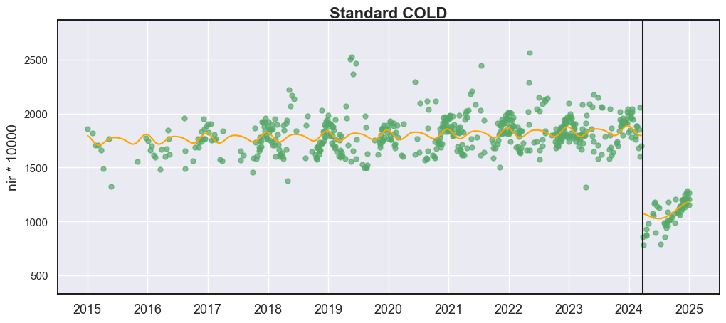
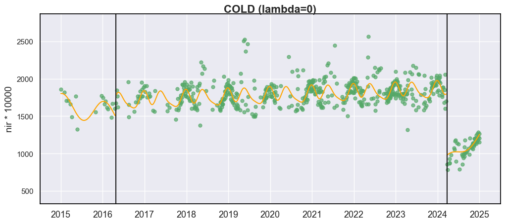
Lambda
您可能对当前的拟合曲线(黄线)不完全满意。为了解决这个问题,我们提供了参数 lam 来控制 Lasso 回归中的正则化程度。当 lam = 0 时,所有谐波系数在无惩罚的情况下进行估计,Lasso 退化为普通最小二乘(OLS)回归。虽然这可能产生对观测数据在视觉上更好的拟合,但会增加过拟合的风险。例如,在下面显示的情况下,在实际火灾干扰之前的 2016 年检测到了一个多余的断点。这个虚假的断点很可能是由曲线拟合过程中的过拟合引起的误检错误。COLD/S-CCD 的默认 lam 为 20,这是基于大量初步测试得出的。
cold_result = cold_detect(dates, blues, greens, reds, nirs, swir1s, swir2s, thermals, qas, lam=0)

# Create figure and axes
fig, ax = plt.subplots(figsize=(12, 5))
# plt.subplots_adjust(left=0.08, right=0.98, top=0.92, bottom=0.1)

display_cold_result(data=np.stack((dates, blues, greens, reds, nirs, swir1s, swir2s, thermals, qas), axis=1), band_names=['blues', 'green', 'red', 'nir', 'swir1', 'swir2', 'thermals'], band_index=3, cold_result=cold_result, axe=ax, title="COLD (lambda=0)")
S-CCD
随机连续变化检测(Stochastic Continuous Change Detection, S-CCD)是连续变化检测与分类(CCDC)框架的一个高级变体(Ye 等人, 2021),旨在提高地表变化检测的时效性和可解释性。与原始 CCDC 对整个 Landsat 或 Harmonized Landsat-Sentinel (HLS) 时间序列拟合确定性谐波和线性模型不同,S-CCD 引入了一种随机更新机制,允许模型随着新的卫星观测数据的到来而动态演化。
S-CCD 的关键创新在于其使用递归模型更新(即卡尔曼滤波),这消除了每当新数据输入时重新拟合整个时间序列的需要。相反,模型系数(趋势和季节参数)以短期记忆的方式增量更新。这种设计使得算法计算效率更高,并且能够近实时运行。此外,S-CCD 允许输出时间序列分量(年际、半年际等)的“状态”,从而除了断点检测外,还能更好地捕捉季节性和总体趋势的渐变。对于回顾性时间序列分析的场景,S-CCD 具有与 COLD 相当的检测精度。
参考文献:
Ye, S., Rogan, J., Zhu, Z., & Eastman, J. R. (2021). A near-real-time approach for monitoring forest disturbance using Landsat time series: Stochastic continuous change detection. Remote Sensing of Environment, 252, 112167.
S-CCD 断点检测
以下是使用 S-CCD 对雅安火灾点的分析:
from pyxccd import sccd_detect

# note that the standard s-ccd doesn't need thermal band for efficient computation, you could switch sccd_detect_flex which allows you to input any combination of bands if you really want to use thermal
sccd_result = sccd_detect(dates, blues, greens, reds, nirs, swir1s, swir2s, qas)

break_date = pd.Timestamp.fromordinal(sccd_result.rec_cg[0]["t_break"]).strftime('%Y-%m-%d')
print(f"The break detected is {break_date}")
sccd_result
The break detected is 2024-03-23
SccdOutput(position=1, rec_cg=array([(735600, 738968, 441, [[ 5.7651807e+03, -7.5955360e+01,  2.8375614e-01,  5.1964793e+00, -2.0415826e+00, -6.4547181e+00], [ 1.6891670e+03, -1.8045355e+01,  2.2810047e+00,  1.6642979e+01, -5.6901956e+00, -1.3014506e+01], [ 1.2292332e+04, -1.6212231e+02,  3.5307232e+01,  1.7814684e+01, -1.0739973e+01, -1.8438562e+01], [-2.6667223e+04,  3.8507657e+02,  9.7016243e+01, -3.8088055e+00,  2.9747089e+01, -5.9461620e+01], [ 2.5863348e+04, -3.3480228e+02,  5.9306335e+01,  2.6777798e+01, -1.2760725e+01, -4.4620617e+01], [ 1.5446797e+04, -2.0042662e+02,  3.9952637e+01,  2.0489840e+01, -1.7458494e+01, -2.8435680e+01]], [28.350677, 33.288532, 34.144318, 94.36975 , 91.12302 , 59.044655], [ 231.40686,  157.6067 ,  277.8084 , -850.01636,  239.03906,  819.48413])],
      dtype={'names': ['t_start', 't_break', 'num_obs', 'coefs', 'rmse', 'magnitude'], 'formats': ['<i4', '<i4', '<i4', ('<f4', (6, 6)), ('<f4', (6,)), ('<f4', (6,))], 'offsets': [0, 4, 8, 12, 156, 180], 'itemsize': 204, 'aligned': True}), min_rmse=array([ 30,  40,  40,  96, 102,  72], dtype=int16), nrt_mode=12, nrt_model=array([], dtype=float64), nrt_queue=array([([ 404,  565,  600,  853, 1293, 1427], 15226),
       ([ 349,  459,  562,  782, 1303, 1422], 15232),
       ([ 350,  469,  592,  879, 1446, 1546], 15247),
       ([ 372,  539,  632,  932, 1353, 1400], 15250),
       ([ 413,  536,  667,  980, 1620, 1683], 15262),
       ([ 434,  578,  724, 1074, 1748, 1785], 15287),
       ([ 596,  656,  762, 1057, 1722, 1675], 15290),
       ([ 555,  684,  811, 1168, 1771, 1698], 15298),
       ([ 483,  634,  806, 1182, 1889, 1822], 15302),
       ([ 321,  466,  605,  897, 1473, 1409], 15305),
       ([ 357,  529,  699, 1137, 1763, 1587], 15312),
       ([ 500,  638,  775, 1130, 1788, 1726], 15327),
       ([ 275,  375,  480,  791, 1327, 1189], 15337),
       ([ 399,  537,  644,  988, 1533, 1439], 15357),
       ([ 389,  485,  566,  858, 1368, 1262], 15362),
       ([ 437,  535,  627,  945, 1464, 1364], 15370),
       ([ 442,  599,  717, 1089, 1623, 1523], 15377),
       ([ 424,  545,  639,  962, 1484, 1412], 15378),
       ([ 410,  558,  662, 1011, 1500, 1386], 15380),
       ([ 493,  647,  779, 1178, 1706, 1578], 15382),
       ([ 409,  565,  681, 1009, 1494, 1386], 15385),
       ([ 247,  467,  634, 1020, 1576, 1462], 15395),
       ([ 430,  586,  699, 1042, 1556, 1423], 15405),
       ([ 424,  588,  715, 1069, 1546, 1400], 15415),
       ([ 240,  411,  537,  989, 1358, 1164], 15420),
       ([ 454,  603,  739, 1206, 1776, 1617], 15427),
       ([ 278,  470,  619, 1088, 1586, 1464], 15435),
       ([ 413,  576,  695, 1091, 1631, 1502], 15440),
       ([ 423,  589,  717, 1073, 1574, 1445], 15445),
       ([ 429,  594,  727, 1122, 1662, 1550], 15447),
       ([ 394,  596,  714, 1137, 1746, 1593], 15450),
       ([ 460,  637,  756, 1138, 1779, 1641], 15458),
       ([ 448,  621,  758, 1099, 1663, 1568], 15460),
       ([ 451,  615,  765, 1121, 1757, 1649], 15462),
       ([ 466,  649,  789, 1120, 1692, 1618], 15465),
       ([ 429,  646,  826, 1198, 1839, 1734], 15466),
       ([ 468,  637,  791, 1154, 1768, 1683], 15467),
       ([ 445,  632,  804, 1199, 1765, 1655], 15470),
       ([ 471,  660,  816, 1206, 1826, 1708], 15472),
       ([ 468,  639,  807, 1155, 1817, 1723], 15477),
       ([ 478,  670,  803, 1132, 1740, 1633], 15480),
       ([ 562,  727,  871, 1243, 1875, 1769], 15482),
       ([ 525,  704,  877, 1268, 1922, 1778], 15490),
       ([ 478,  666,  848, 1209, 1864, 1749], 15492),
       ([ 490,  690,  853, 1185, 1769, 1691], 15495),
       ([ 468,  691,  903, 1283, 1955, 1844], 15498),
       ([ 478,  673,  860, 1225, 1810, 1724], 15500),
       ([ 516,  692,  875, 1265, 1947, 1818], 15506),
       ([ 483,  668,  854, 1206, 1880, 1770], 15507),
       ([ 464,  657,  822, 1153, 1758, 1658], 15510)],
      dtype={'names': ['clry', 'clrx_since1982'], 'formats': [('<i2', (6,)), '<i2'], 'offsets': [0, 12], 'itemsize': 14, 'aligned': True}))
S-CCD 和 COLD 都将干扰检测为 ‘2024-03-23’。实际上,我已经测试了很多案例。对于回顾性分析,S-CCD 和 COLD 通常产生非常相似的断点检测结果。
S-CCD 的输出是一个结构化对象,包含六个元素。
元素 |
数据类型 |
描述 |
|---|---|---|
position |
int |
当前像素的位置,通常编码为 10000*行号+列号 |
rec_cg |
ndarray |
通过回顾性突变检测得到的时序片段 |
nrt_mode |
int |
当前模式:第一位数字表示可预测性,第二位表示
|
nrt_model |
ndarray |
最后一段的近实时模型,将会递归更新 |
nrt_queue |
ndarray |
当 |
min_rmse |
ndarray |
CCDC 中的最小均方根误差,用于避免来自黑体的过度检测 |
其中,rec_cg 存储通过断点检测识别的历史时间段的结果。与 COLD 算法的一个关键区别在于对 rec_cg 最后一个时间段的处理:在 S-CCD 中,这个时间段要么保存到 nrt_model,要么保存到 nrt_queue 用于近实时(NRT)应用。因此,检测到的断点数量等于记录的时间段数量。最后一个时间段的分配取决于像元的状态,该状态由变量 nrt_mode 指示。具体来说:
如果最后一个时间段的初始模型已经构建,则
nrt_mode的第二位是 1(正常情况)或 3(雪况)。在这种情况下,时间段存储在nrt_model中,而nrt_queue保持为空。如果初始模型尚未构建,则
nrt_mode的第二位是 2(正常情况)或 4(雪况)。在这种情况下,nrt_queue开始存储新的观测数据,直到有足够的数据来初始化模型,而 nrt_model 保持为空。
这种设计确保 S-CCD 能够灵活处理已充分初始化的时间段和新兴的时间段,这对于及时准确的近实时干扰监测至关重要。我们将在第 7 课中介绍这种设计的细节。
使用 S-CCD 进行 NRT 场景的细节将在第 7 课中看到。在本课中,我们将重点关注基于 S-CCD 的回顾性分析。
### S-CCD 可视化
from pyxccd.common import SccdOutput
from pyxccd.utils import getcategory_sccd, defaults

def display_sccd_result(
    data: np.ndarray,
    band_names: List[str],
    band_index: int,
    sccd_result: SccdOutput,
    axe: Axes,
    title: str = 'S-CCD',
    plot_kwargs: Optional[Dict] = None
) -> Tuple[plt.Figure, List[plt.Axes]]:
    """
    Compare COLD and SCCD change detection algorithms by plotting their results side by side.

    This function takes time series remote sensing data, applies both COLD and SCCD algorithms,
    and visualizes the curve fitting and break detection results for comparison.

    Parameters:
    -----------
    data : np.ndarray
        Input data array with shape (n_observations, n_bands + 2) where:
        - First column: ordinal dates (days since January 1, AD 1)
        - Next n_bands columns: spectral band values
        - Last column: QA flags (0-clear, 1-water, 2-shadow, 3-snow, 4-cloud)

    band_names : List[str]
        List of band names corresponding to the spectral bands in the data (e.g., ['red', 'nir'])

    band_index : int
        1-based index of the band to plot (e.g., 0 for first band, 1 for second band)

    sccd_result: SccdOutput
        Output of sccd_detect

    axe: Axes
        An Axes object represents a single plot within that Figure

    title: Str
        The figure title. The default is "S-CCD"

    plot_kwargs : Dict, optional
        Additional keyword arguments to pass to the display function. Possible keys:
        - 'marker_size': size of observation markers (default: 5)
        - 'marker_alpha': transparency of markers (default: 0.7)
        - 'line_color': color of model fit lines (default: 'orange')
        - 'font_size': base font size (default: 14)

    Returns:
    --------
    Tuple[plt.Figure, List[plt.Axes]]
        A tuple containing the matplotlib Figure object and a list of Axes objects
        (top axis is COLD results, bottom axis is SCCD results)

    """
    w = np.pi * 2 / 365.25

    # Set default plot parameters
    default_plot_kwargs: Dict[str, Union[int, float, str]] = {
        'marker_size': 5,
        'marker_alpha': 0.7,
        'line_color': 'orange',
        'font_size': 14
    }
    if plot_kwargs is not None:
        default_plot_kwargs.update(plot_kwargs)

    # Extract values with proper type casting
    font_size = default_plot_kwargs.get('font_size', 14)
    try:
        title_font_size = int(font_size) + 2
    except (TypeError, ValueError):
        title_font_size = 16


    # Clean and prepare data
    data = data[np.all(np.isfinite(data), axis=1)]
    data_df = pd.DataFrame(data, columns=['dates'] + band_names + ['qa'])


    # Plot COLD results
    w = np.pi * 2 / 365.25
    slope_scale = 10000

    # Prepare clean data for COLD plot
    data_clean = data_df[(data_df['qa'] == 0) | (data_df['qa'] == 1)].copy()
    data_clean =  data_clean[(data_clean >= 0).all(axis=1) & (data_clean.drop(columns="dates") <= 10000).all(axis=1)]
    calendar_dates = [pd.Timestamp.fromordinal(int(row)) for row in data_clean["dates"]]
    data_clean.loc[:, 'dates_formal'] = calendar_dates

    # Calculate y-axis limits
    band_name = band_names[band_index]
    band_values = data_clean[data_clean['qa'] == 0 | (data_clean['qa'] == 1)][band_name]
    # band_values  = band_values[band_values <10000]
    q01, q99 = np.quantile(band_values, [0.01, 0.99])
    extra = (q99 - q01) * 0.4
    ylim_low = q01 - extra
    ylim_high = q99 + extra

    # Plot SCCD observations
    axe.plot(
        'dates_formal', band_name, 'go',
        markersize=default_plot_kwargs['marker_size'],
        alpha=default_plot_kwargs['marker_alpha'],
        data=data_clean
    )

    # Plot SCCD segments
    for segment in sccd_result.rec_cg:
        j = np.arange(segment['t_start'], segment['t_break'] + 1, 1)
        if len(segment['coefs'][band_index]) == 8:
            plot_df = pd.DataFrame(
                {
                'dates': j,
                'trend': j * segment['coefs'][band_index][1] / slope_scale + segment['coefs'][band_index][0],
                'annual': np.cos(w * j) * segment['coefs'][band_index][2] + np.sin(w * j) * segment['coefs'][band_index][3],
                'semiannual': np.cos(2 * w * j) * segment['coefs'][band_index][4] + np.sin(2 * w * j) * segment['coefs'][band_index][5],
                'trimodal': np.cos(3 * w * j) * segment['coefs'][band_index][6] + np.sin(3 * w * j) * segment['coefs'][band_index][7]
            })
        else:
            plot_df = pd.DataFrame(
                {
                'dates': j,
                'trend': j * segment['coefs'][band_index][1] / slope_scale + segment['coefs'][band_index][0],
                'annual': np.cos(w * j) * segment['coefs'][band_index][2] + np.sin(w * j) * segment['coefs'][band_index][3],
                'semiannual': np.cos(2 * w * j) * segment['coefs'][band_index][4] + np.sin(2 * w * j) * segment['coefs'][band_index][5],
                'trimodal': j * 0
            })
        plot_df['predicted'] = (
            plot_df['trend'] +
            plot_df['annual'] +
            plot_df['semiannual']+
            plot_df['trimodal']
        )

        # Convert dates and plot model fit
        calendar_dates = [pd.Timestamp.fromordinal(int(row)) for row in plot_df["dates"]]
        plot_df.loc[:, 'dates_formal'] = calendar_dates
        g = sns.lineplot(
            x="dates_formal", y="predicted",
            data=plot_df,
            label="Model fit",
            ax=axe,
            color=default_plot_kwargs['line_color']
        )
        if g.legend_ is not None:
            g.legend_.remove()

    # Plot near-real-time projection for SCCD if available
    if hasattr(sccd_result, 'nrt_mode') and (sccd_result.nrt_mode %10 == 1 or sccd_result.nrt_mode == 3 or sccd_result.nrt_mode %10 == 5):
        recent_obs = sccd_result.nrt_model['obs_date_since1982'][sccd_result.nrt_model['obs_date_since1982']>0]
        j = np.arange(
            sccd_result.nrt_model['t_start_since1982'] + defaults['COMMON']['JULIAN_LANDSAT4_LAUNCH'],
            recent_obs[-1]+ defaults['COMMON']['JULIAN_LANDSAT4_LAUNCH']+1,
            1
        )

        if len(sccd_result.nrt_model['nrt_coefs'][band_index]) == 8:
            plot_df = pd.DataFrame(
                {
                'dates': j,
                'trend': j * sccd_result.nrt_model['nrt_coefs'][band_index][1] / slope_scale + sccd_result.nrt_model['nrt_coefs'][band_index][0],
                'annual': np.cos(w * j) * sccd_result.nrt_model['nrt_coefs'][band_index][2] + np.sin(w * j) * sccd_result.nrt_model['nrt_coefs'][band_index][3],
                'semiannual': np.cos(2 * w * j) * sccd_result.nrt_model['nrt_coefs'][band_index][4] + np.sin(2 * w * j) * sccd_result.nrt_model['nrt_coefs'][band_index][5],
                'trimodal': np.cos(3 * w * j) * sccd_result.nrt_model['nrt_coefs'][band_index][6] + np.sin(3 * w * j) * sccd_result.nrt_model['nrt_coefs'][band_index][7]
            })
        else:
            plot_df = pd.DataFrame(
                {
                'dates': j,
                'trend': j * sccd_result.nrt_model['nrt_coefs'][band_index][1] / slope_scale + sccd_result.nrt_model['nrt_coefs'][band_index][0],
                'annual': np.cos(w * j) * sccd_result.nrt_model['nrt_coefs'][band_index][2] + np.sin(w * j) * sccd_result.nrt_model['nrt_coefs'][band_index][3],
                'semiannual': np.cos(2 * w * j) * sccd_result.nrt_model['nrt_coefs'][band_index][4] + np.sin(2 * w * j) * sccd_result.nrt_model['nrt_coefs'][band_index][5],
                'trimodal': j * 0
            })

        plot_df['predicted'] = plot_df['trend'] + plot_df['annual'] + plot_df['semiannual']+ plot_df['trimodal']
        calendar_dates = [pd.Timestamp.fromordinal(int(row)) for row in plot_df["dates"]]
        plot_df.loc[:, 'dates_formal'] = calendar_dates
        g = sns.lineplot(
            x="dates_formal", y="predicted",
            data=plot_df,
            label="Model fit",
            ax=axe,
            color=default_plot_kwargs['line_color']
        )
        if g.legend_ is not None:
            g.legend_.remove()

    # Plot breaks
    for i in range(len(sccd_result.rec_cg)):
        if getcategory_sccd(sccd_result.rec_cg, i) == 1:
            axe.axvline(pd.Timestamp.fromordinal(sccd_result.rec_cg[i]['t_break']), color='k')
        else:
            axe.axvline(pd.Timestamp.fromordinal(sccd_result.rec_cg[i]['t_break']), color='r')

    axe.set_ylabel(f"{band_name} * 10000", fontsize=default_plot_kwargs['font_size'])

    # Handle tick params with type safety
    tick_font_size = default_plot_kwargs['font_size']
    if isinstance(tick_font_size, (int, float)):
        axe.tick_params(axis='x', labelsize=int(tick_font_size)-1)
    else:
        axe.tick_params(axis='x', labelsize=13)  # fallback

    axe.set(ylim=(ylim_low, ylim_high))
    axe.set_xlabel("", fontsize=6)

    # Format spines
    for spine in axe.spines.values():
        spine.set_edgecolor('black')
    title_font_size = int(font_size) + 2 if isinstance(font_size, (int, float)) else 16
    axe.set_title(title, fontweight="bold", size=title_font_size, pad=2)

sns.set_theme(style="darkgrid")
sns.set_context("notebook")

# Create figure and axes
fig, ax = plt.subplots(figsize=(12, 5))

display_sccd_result(data=np.stack((dates, blues, greens, reds, nirs, swir1s, swir2s, qas), axis=1), band_names=['blues', 'green', 'red', 'nir', 'swir1', 'swir2'], band_index=3, sccd_result=sccd_result, axe=ax)
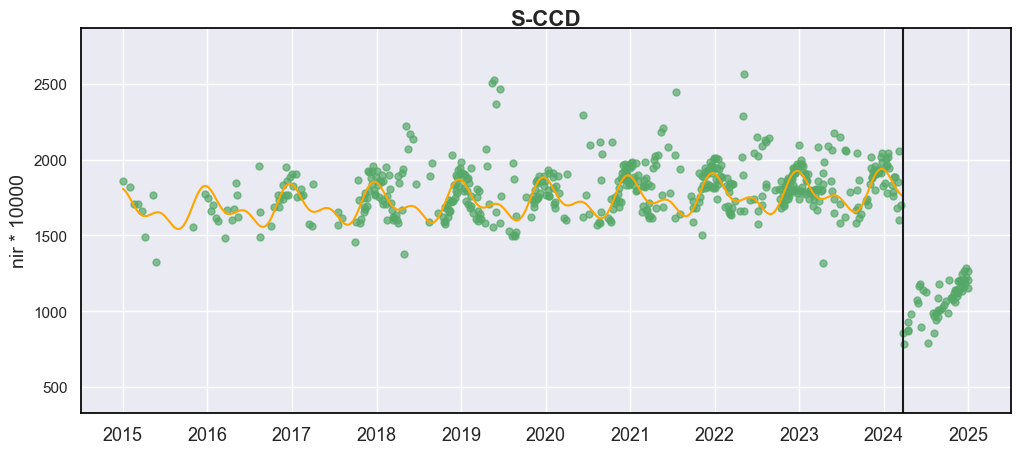
从结果来看,S-CCD 产生了与 COLD 非常相似的结果。对于最后一个时间段,没有拟合曲线,这是因为 nrt_model 由于观测数据不足(<=18)或观测周期不到一年而尚未初始化。
好的。到目前为止,您已经学习了第一课,运行基本的 COLD 和 S-CCD 算法进行干扰检测。如果变化太微妙而无法检测到断点怎么办?下一课将引导您调整算法参数以提高灵敏度。